Automated Testing of Simulation Code via Hypothesis Testing
Missing a Theory of Testing for Scientific Code
If you search the Internet for resources on the theory of testing code, you will find information about the different types of tests and how to write them. You will also find that it is generally accepted among programmers that good code is tested and bad code is not. The problem for scientists and engineers, however, is that the theory concerning the testing of computer code was developed primarily by programmers that work on systems that model business processes. There is little theory on how, for example, to test the outcome of physics simulations. To further exacerbate the problem, scientific programmers feel obliged to write tests without the guidance of such a theory because of the imperative to test their code. This leads to convoluted tests that are difficult to understand and maintain.
Scientific Code is Different
Code that models business processes is based on explicit rules that are developed from a set of requirements. An example of a rule that a business system might follow is "If a customer has ordered an item and has not paid, then send her an invoice."
To test the above rule, we write out all the possible cases and write a test for each one. For example:
- A customer orders an item without paying. Expected result: an invoice is sent.
- A customer orders an item and pays at the time of checkout: Expected result: no invoice is sent.
I have found that a good way to identify test cases in business logic is to look for if/else statements in a rule. Each branch of the statement should be a different test.
Now let's consider a physics simulation. I am an optical engineer, so I will use an example from optics. One thing I have often done in my work is to simulate the image formation process of a lens system, including the noise imparted by the camera. A simple model of a CMOS camera pixel is one that takes an input signal in photons, adds shot noise, converts it to photoelectrons, adds dark noise, and then converts the electron signal into analog-to-digital units. Schematically:
photons --> electrons --> ADUs
A simplified Python code snippet that models this process, including noise, is below. An instance of the camera class has a method called snap that takes input array of photons and converts it to ADUs.
from dataclasses import dataclass

import numpy as np


@dataclass
class Camera:
    baseline: int = 100  # ADU
    bit_depth: int = 12
    dark_noise: float = 6.83  # e-
    gain: float = 0.12  # ADU / e-
    quantum_efficiency: float = 0.76
    well_capacity: int = 32406  # e-
    rng: np.random.Generator = np.random.default_rng()

    def snap(self, signal):
        # Simulate shot noise and convert to electrons
        photoelectrons = self.rng.poisson(
            self.quantum_efficiency * signal, size=signal.shape
        )

        # Add dark noise
        electrons = (
            self.rng.normal(scale=self.dark_noise, size=photoelectrons.shape)
            + photoelectrons
        )

        # Clip to the well capacity to model electron saturation
        electrons = np.clip(electrons, 0, self.well_capacity)

        # Convert to ADU
        adu = electrons * self.gain + self.baseline

        # Clip to the bit depth to model ADU saturation
        adu = np.clip(adu, 0, 2 ** self.bit_depth - 1)

        return adu.astype(np.uint16)
How can we test this code? In this case, there are no if/else statements to help us identify test cases. Some possible solutions are:
-
An expert can review it. But what if we don't have an expert? Or, if you are an expert, how do we know that we haven't made a mistake? I have worked professionally as both an optical and a software engineer and I can tell you that I make coding mistakes many times a day. And what if the simulation is thousands of lines of code? This solution, though useful, cannot be sufficient for testing.
-
Compute what the results ought to be for a given set of inputs. Rules like "If the baseline is 100, and the bit depth is 12, etc., then the output is 542 ADU" are not that useful here because the output is random.
-
Evaluate the code and manually check that it produces the desired results. This is similar to expert review. The problem with this approach is that you would need to recheck the code every time a change is made. One of the advantages of testing business logic is that the tests can be automated. It would be advantageous to preserve automation in testing scientific code.
-
We could always fix the value of the seed for the random number generator to at least make the test deterministic, but then we would not know whether the variation in the simulation output is what we would expect from run-to-run. I'm also unsure whether the same seed produces the same results across different hardware architectures. Since the simulation is non-deterministic at its core, it would be nice to include this attribute within the test case.
Automated Testing of Simulation Results via Hypothesis Testing
The solution that I have found to the above-listed problems is derived from ideas that I learned in a class on quality control that I took in college. In short, we run the simulation a number of times and compute one or more statistics from the results. The statistics are compared to their theoretical values in a hypothesis test, and, if the result is outside of a given tolerance, the test fails. If the probability of failure is made small enough, then a failure of the test practically indicates an error in the simulation code rather than a random failure due to the stochastic output.
Theoretical Values for Test Statistics
In the example of a CMOS camera, both the theoretical mean and the variance of a pixel are known. The EMVA 1288 Linear Model states that
$$ \mu_y = K \left( \eta \mu_p + \mu_d \right) + B $$
where \( \mu_y \) is the mean ADU count, \( K \) is the gain, \( \eta \) is the quantum efficiency, \( \mu_p \) is the mean photon count, \( \mu_d \) is the mean dark noise, and \( B \) is the baseline value, i.e. the average ADU count under no illumination. Likewise, the variance of the pixel describes the noise:
$$ \sigma_y = \sqrt{K^2 \sigma_d^2 + \sigma_q^2 + K \left( \mu_y - B \right)} $$
where \( \sigma_y \) is the standard deviation of the ADU counts, \( \sigma_d^2 \) is the dark noise variance, and \( \sigma_q^2 = 1 / 12 \, \text{ADU} \) is the quantization noise, i.e. the noise from converting an analog voltage into discrete ADU values.
Hypothesis Testing
We can formulate a hypothesis test for each test statistic. The test for each is:
- Null hypothesis : the simulation statistics and the theoretical values are the same
- Alternative hypothesis : the simulation statistics and the theoretical values are different
Let's first focus on the mean pixel values. To perform this hypothesis test, I ran the simulation code a number of times. For convenience, I chose an input signal of 1000 photons. Here's the resulting histogram:
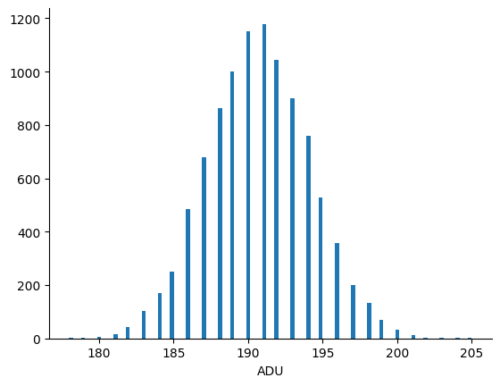
The mean of this distribution is 190.721 ADU and the standard deviation is 3.437 ADU. The theoretical values are 191.2 ADU and 3.420 ADU, respectively. Importantly, if I re-run the simulation, then I get a different histogram because the simulation's output is random.
The above histogram is called the sampling distribution of the mean, and its width is proportional to the standard error of the mean. (Edit 2024/05/30 Actually, I think I am wrong here. This is not the sampling distribution of the mean. To get it we would need to repeat the above experiment a number of times and compute the mean each time, much like I do in the following section. The set of all means from doing so would be its sampling distribution. Fortunately, the estimate of the confidence intervals in what follows should still hold because the sampling distribution of the mean tends to a normal distribution for large \(N \), and this allows for the expression in the equation that follows.)
Hypothesis Testing of the Mean Pixel Value
To perform the hypthosesis test on the mean, I build a confidence interval around the simulated value using the following formula:
$$ \mu_y \pm X \frac{s}{\sqrt{N}} $$
Here \( s \) is my estimated standard deviation (3.437 ADU in the example above), and \( N = 10,000 \) is the number of simulated values. Their ratio \( \frac{s}{\sqrt{N}} \) is an estimate of the standard error of the mean. \( X \) is a proportionality factor that is essentially a tolerance on how close the simulated value must be to the theoretical one to be considered "equal". A larger tolerance means that it is less likely that the hypothesis test will fail, but I am less certain that the value of the simulation is exactly equal to the theoretical value.
If this looks familiar, it should. In introductory statistics classes, this approach is called Student's one sample t-test. In the t-test, the value for \( X \) is denoted as \( t \) and depends on the desired confidence level and on the number of data points in the sample. (Strictly speaking, it's the number of data points minus 1.)
As far as I can tell there's no rule for selecting a value of \( X \); rather, it's a free parameter. I often choose 3. Why? Well, if the sampling distribution is approximately normally distributed, and the number of sample points is large, then the theoretical mean should lie within 3 standard errors of the simulated one approximately 99.7% of the time if the algorithm is correct. Alternatively, this means that a correct simulation will produce a result that is more than three standard errors from the theoretical mean about every 1 out of 370 test runs.
Hypothesis Testing of the Noise
Recall that standard deviation of pixel values is a measure of the noise. The approach to testing it remains the same as before. We write the confidence interval as
$$ \sigma_y \pm X \left( s.e. \right) $$
where we have \( s.e. \) as the standard error of the standard deviation. If the simulated standard deviation is outside this interval, then we reject the null hypothesis and fail the test.
Now, how do we calculate the standard error of the standard deviation? Unlike with the mean value, we have only one value for the standard deviation of the pixel values. Furthermore, there doesn't seem to be a simple formula for the standard error of the variance or standard error of the standard deviation. (I looked around the Math and Statistics Stack Exchanges, but what I did find produced standard errors that were way too large.)
Faced with this problem, I have two options:
- run the simulation a number of times to get a distribution of standard deviations
- draw pixel values from the existing simulation data with replacement to estimate the sampling distribution. This approach is known as bootstrapping.
In this situation, both are valid approaches because the simulation runs quite quickly. However, if the simulation is slow, bootstrapping might be desirable because resampling the simulated data is relatively fast.
I provide below a function that makes a bootstrap estimate of the standard error of pixel values to give you an idea of how this works. It draws n samples from the simulated pixel values with replacement and places the results in the rows of an array. Then, the standard devation of each row is computed. Finally, since the standard error is the standard deviation of the sampling distribution, the standard deviation of resampled standard deviations is computed and returned.
def se_std(data, n = 1000) -> float:
    samples = np.random.choice(data.ravel(), (n, data.size), replace=True)
    std_sampling_distribution = samples.std(axis=1)

    return np.std(std_sampling_distribution)
Of course, the value of n in the function above is arbitrary. From what I can tell, setting n to be the size of the data is somewhat standard practice.
Automated Hypothesis Testing
At this point, we can calculate the probability that the mean and standard deviation of the simulated pixel values will lie farther than some distance from their theoretical values. This means that we know roughly how often a test will fail due to pure luck.
To put these into an automated test function, we need only translate the two hypotheses into an assertion. The null hypothesis should correspond to the argument of the assertion being true; the alternative hypothesis corresponds to a false argument.
TOL = 3

def test_cmos_camera(camera):
    num_pixels = 32, 32
    mean_photons = 100
    photons = (mean_photons * np.ones(num_pixels)).astype(np.uint8)
    expected_mean = 191.2
    expected_std = 3.42

    img = camera.snap(photons)

    tol_mean = TOL * img.std() / np.sqrt(num_pixels[0] * num_pixels[1])
    tol_std = TOL * se_std(img)

    assert np.isclose(img.mean(), expected_mean, atol=tol_mean)
    assert np.isclose(img.std(), expected_std, atol=tol_std)
With a TOL value of 3 and with the sampling distributions being more-or-less normally distributed, each assertion should fail about 1 / 370 times because the area in the tails of the distribution beyond three standard errors is 1 / 370. We can put this test into our test suite and continuous integration (CI) system and run it automatically using whatever tools we wish, e.g. GitHub Actions and pytest.
Discussion
Non-deterministic Tests
It is an often-stated rule of thumb that automated tests should never fail randomly because it makes failures difficult to diagnose and makes you likely to ignore the tests. Here however it is in the very nature of this test that it will fail randomly from time to time. What are we to do?
An easy solution would be to isolate these sorts of tests and run them separately from the deterministic ones so that we know exactly where the error occurred. Then, if there is a failure of the non-deterministic tests, the CI could just run them again. If TOL is set so that a test failure is very rare, then any failure of these tests twice would practically indicate a failure of the algorithm to produce the theoretical results.
Testing Absolute Tolerances
It could be argued that what I presented here is a lot of work just to make an assertion that a simulation result is close to a known value. In other words, it's just a fancy way to test for absolute tolerances, and possibly is more complex than it needs to be. I can't say that I entirely disagree with this.
As an alternative, consider the following: if we run the simulation a few times we can get a sense of the variation in its output, and we can use these values to roughly set a tolerance that states by how much the simulated and theoretical results should differ. This is arguably faster than constructing the confidence intervals like we did above.
The value in the hypothesis testing approach is that you can know the probability of failure to a high degree of accuracy. Whether or not this is important probably depends on what you want to do, but it does provide you with a deeper understanding of the behavior of the simulation that might help debug difficult problems.
Testing for Other Types of Errors
There are certainly other problems in testing simulation code that are not covered here. The above approach won't tell you directly if you have entered an equation incorrectly. It also requires theoretical values for the summary statistics of the simulation's output. If you have a theory for these already, you might argue that a simulation would be superfluous.
If it's easy to implement automated tests for your simulation that are based on hypothesis testing, and if you expect the code to change often, then having a few of these sorts of tests will at least provide you a degree of confidence that everything is working as you expect as you make changes. And that is one of the goals of having automated tests: fearless refactoring.
Testing the Frequency of Failures
I stated often that with hypothesis testing we know how often the code should fail, but we never actually tested that. We could have run the simulation a large number of times and verified that the number of failures was approximately equal to the theoretical number of failures.
To my mind, it seems that this is just the exact same problem that was addressed above, but instead of testing summary statistics on the output values we test the number of failures. And since the number of failures will vary randomly, we would need a sampling distribution for this. So really this approach requires more CPU clock cycles to do the same thing because we need to run the simulation a large number of times.
Summary
- Automated testing of simulation code is different than testing business logic due to its stochastic nature and inability to be reduced to "rules"
- We can formulate hypothesis tests to determine how often the simulation produces values that are farther than a given distance from what theory predicts
- The hypothesis tests can be translated into test cases: accepting the null hypothesis means the test passes, whereas rejecting the null hypothesis means the test fails
- Non-deterministic testing is useful when it is quick to implement and you expect to change the code often
Comments
Comments powered by Disqus