In my last post I covered some basic mathematics of radiometry. I realized shortly after writing the post that there was still a topic that I did not fully understand but that is central to radiometry and illumination optics in particular: Lambert's cosine law. According to Wikipedia, this law states:

the observed radiant intensity or luminous intensity from an ideal diffusely reflecting surface or ideal diffuse radiator is directly proportional to the cosine of the angle θ between the observer's line of sight and the surface normal; I = I0 cos θ.

The dependence of the intensity on \( \cos \theta \) is mathematically the same as the dependence of the projected area of a surface patch when viewed at an angle, a term known as foreshortening. In my previous post I had described foreshortening of remote surface patches, but not emitters. In effect, I had only described foreshortening as an effect concerning detection, but in reality it concerns emission as well. I very quickly ran into a conceptual problem when trying to apply the concept to emitters. The solution to this problem turns out to be quite... illuminating. (Ha ha.)

Ideal Emitters

I'll start by breaking down Wikipedia's definition of the cosine law. First, it deals with ideal, diffuse reflecting and radiating surfaces. For now, I'll limit the discussion to just radiating surfaces.

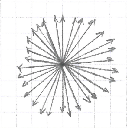
So what is an ideal radiating surface? It is one that can be described as a collection of mutually incoherent point sources radiating light equally in all directions. (Or so I thought.) A single point source radiating equally in all directions would look like this:

Here, each ray carries the same amount of power, and the number of rays per solid angle is constant. The length of a ray doesn't mean anything since, strictly speaking, a ray extends an infinite distance from the source.

Radiant Intensity

An ideal emitter is just a set of ideal point sources. Since the individual point sources are extended across space, we often call such a source an extended source.

Now, since each ray carries the same amount of power, then the set of all rays traveling in the same direction represents the total power emitted into that direction.

But the power emitted by a source as a function of direction is the radiant intensity of the emitter. So we can think of radiant intensity as the sum over the powers carried by all the rays traveling in the same direction from the source.

The angular distribution of the radiant intensity of an emitter, therefore, is a purely geometrical construction.

Point Sources on a Surface or in a Volume?

The Problem

Here's where I ran into my problem. I knew that LEDs could be modeled as Lambertian emitters to a decent degree of accuracy. This means that their radiant intensity should fall off like \( \cos \theta \) where \( \theta \) is the angle between the direction being considered and the normal to the surface. As described in the previous section, I also knew that the number of rays in a given direction should be proportional to the power emitted into that direction. So after counting the rays emitted into each direction, I should find that this number falls off as \( \cos \theta \).

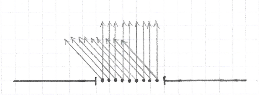
But when I sketched a picture of an LED as a collection of ideal emitters on a surface, I got the following:

I've drawn rays in only two different directions, but you can see that the number of rays remains the same regardless of direction. So there's an inconsistency here. Where is it?

The Qualitative Solution

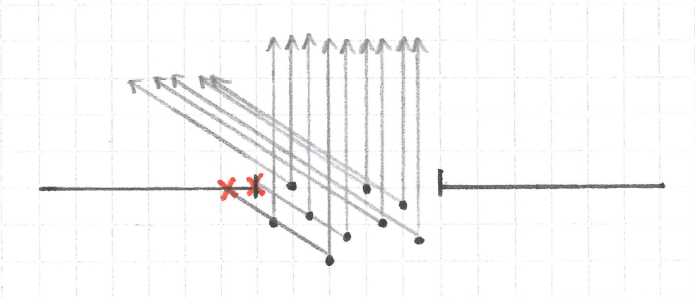
It took me a while to realize that the problem was with my conceptual model of the LED as a collection of emitters on a surface. A small hole in a black body radiator is also a Lambertian emitter. But a black body is a volume, not a surface. If instead I think of the LED as a window into a volume of ideal point sources, then I can see that all the rays behind the window and in the forward direction pass through the window. A fraction of the rays at any other direction are blocked, which results in a decrease in the amount of power emitted into their direction. And finally, the number of rays that are blocked increases as the angle away from the normal increases.

Derivation of Lambert's Cosine Law

In what follows I used Claude to help me set up the derivation, but have validated it myself.

The Setup

I say that this is a qualitative solution because it doesn't actually derive the \( \cos \theta \) dependence. As it turns out, the actual derivation is subtle and requires that we impose another condition onto the medium inside the LED.

First, fill the half space \( z < 0 \) with \( n \) isotropic emitters per unit volume. Then, put an opaque screen at \( z = 0 \) with a window of area \( A \). Note that the emitters now extend beyond the \( x, y \) extent of the window, unlike what I drew above.

Rigorous Ray Counting

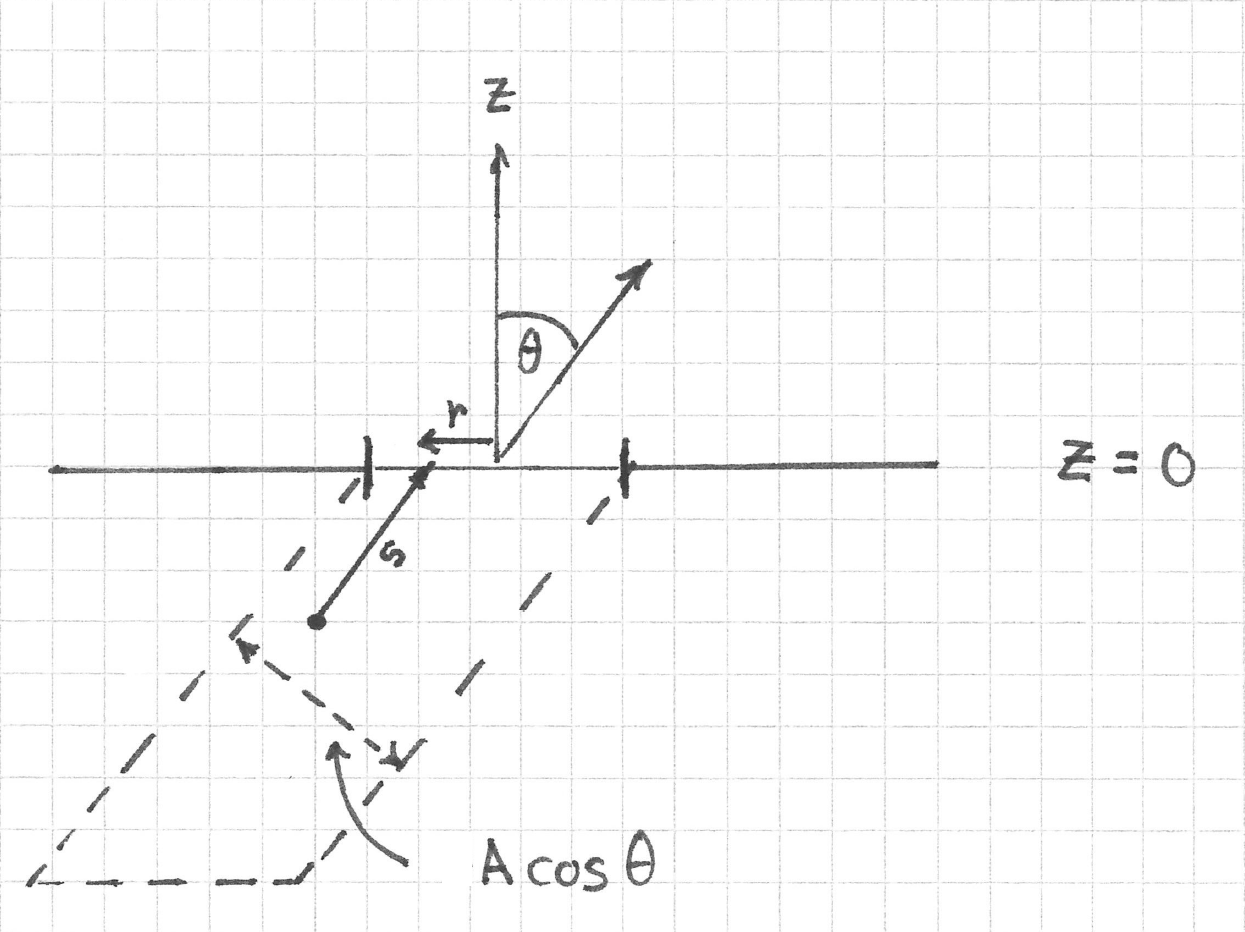
Next, we need a way to count the number of rays leaving the window in direction \( \theta \). To do this, I'm actually going to map each ray to its source point and count the number of source points instead. Let \( \hat{d} \) represent the unit vector corresponding to direction \( \theta \). Its elements are just the direction cosines of each ray. Also, let \( r \) represent the distance from the origin to the point where the ray intersects the window. \( \vec{r} \) ranges over the window, and \(dA\) is its area element. Finally, let \( s \) represent the distance along the ray to the source point. This leads to the familiar parametric representation of a ray used by ray tracers:

$$ \vec{p} = \vec{r} - s \hat {d} $$

I've used the negative sign because I'm tracing backwards into the medium, and the magnitude of \( \vec{r} \) is just \( r \).

As seen in the figure below, the set of all source points inside the medium whose rays travel in direction \( \theta \) and that also exit the window fills a volume whose differential element is \( dV = \cos \theta dA \, ds \).

If each source point emits a total power \( P \) into a solid angle of \( 4 \pi \) steradians, then the intensity as a function of \( \theta \) is

$$ I ( \theta ) = \frac{n P}{4 \pi} \int_{window} \cos \theta \, dA \int_{s=0}^{\infty} ds = \infty . $$

Oops.

Preventing Infinite Intensity

The thing which prevents the power from blowing up is absorption by the medium. Let \( \alpha \) represent the Lambert-Beer absorption coefficient of the LED material. Then the power carried along a ray is attenuated by a factor \( \exp \left(- \alpha s \right) \) after a path length \(s \) inside the material. The integral for intensity as a function of \( \theta \) is now

$$ I ( \theta) = \frac{n P}{4 \pi} \int_{window} \cos \theta \, dA \int_{s=0}^{\infty} \exp \left( - \alpha s \right) ds = \frac{n P}{4 \pi \alpha} A \cos \theta. $$

This is exactly Lambert's cosine law, with \( I_0 = \frac{n P}{4 \pi \alpha} A \).

Some Final Observations

I can go a bit further. Dividing out the projected area \( A \cos \theta \) gives the radiance, which is independent of angle:

$$ L = \frac{n P}{4 \pi \alpha}. $$

This has units of power per area per solid angle, as it should.

I was genuinely surprised to learn how important absorption is to deriving Lambert's cosine law. If the material did not absorb but had a finite thickness \( D \) (to prevent the integral from blowing up), then the integral over path length would be \( D / \cos \theta \). The cosine in the denominator would cancel the one from the projected area of the window. The radiance would furthermore increase towards larger angles like \( 1 / \cos \theta \). In other words, it would no longer be constant.

Finally, I think it's interesting that, under this conceptual setup, Lambert's cosine law is still just foreshortening of a patch when viewed at an angle. The difference is that this time we're looking at the patch/window from inside the LED material.

I have two projects at the moment that involve modeling radiometric quantities in optical systems. At the outset of these projects I felt that I needed to refresh my knowledge of the basics. This post contains my notes about the topics that I think form the mathematical foundation of radiometry.

Spherical Coordinate Systems

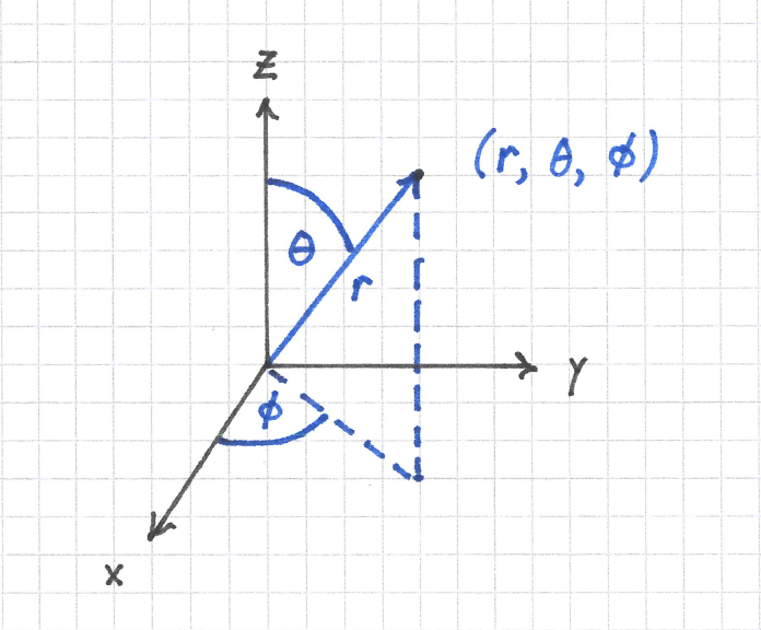
Radiometric models are most naturally constructed in spherical coordinate systems. A spherical coordinate system is illustrated below.

In the above illustration, I use the physicist's notation to denote:

1. \( r \) : the radial coordinate
2. \( \theta \) : the polar (or zenith) angle
3. \( \phi \) : the azimuthal angle

The Differential Volume Element

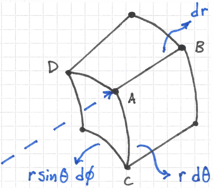
The differential volume element in spherical coordinates is constructed as follows.

In the figure above, the point \( A \) represents the point \( \left( r, \theta, \phi \right) \) in spherical coordinates.

1. The line segment \( AB \) has length \( dr \)
2. The arc \( AC \) has length \( r \, d \theta \)
3. The arc \( AD \) has length \( r \sin \theta \, d \phi \)

The differential volume element therefore is

$$ dV = r^2 \sin \theta \, dr \, d \theta \, d \phi $$.

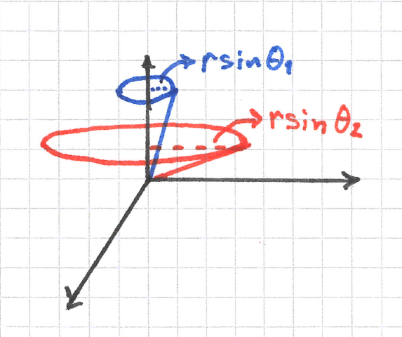
The reason for the \( \sin \theta \) term is that the ray from the origin to the point \( \left( r, \theta, \phi \right) \) traces out a circle of radius \( r \sin \theta \) when I let \( \phi \) vary from 0 to \( 2 \pi \) as illustrated below:

Solid Angle

A central concept in radiometry is the idea of the solid angle. Solid angle is the equivalent to angle in 3D space and is represented by the Greek letter \( \Omega \).

We use solid angle to describe the apparent size of a surface as reviewed from some point in space. For a differential surface patch that we denote \( dS \) at a distance \( r \) from the point of observation \( P \), we say that the differential solid angle subtended by the patch at \( P \) is

$$ d \Omega = \sin \theta \, d \theta \, d \phi $$.

A good heuristic to remember this quantity is to take the volume element in spherical coordinates and divide by \( r^2 \, dr \).

I often see the definition \( \Omega = A / r^2 \), but this applies in the special case when the patch has area \( A \) and is a subset of the surface of a sphere of radius \( r \). More generally, if \( dS' \) represents the projected surface area of a patch, then

$$ d \Omega = \frac{dS'}{r^2} $$.

Why must \( dS' \) be a projected area? The answer is due to an effect known as foreshortening, which will be discussed in the next section.

When the observation point is at the origin and I use spherical coordinates, then I can equate the two expressions above:

$$ d \Omega = \frac{dS'}{r^2} = \sin \theta \, d \theta \, d \phi $$

Foreshortening

If the patch is oriented such that its unit normal vector \( \hat{n} \) is at an angle \( \theta \) to the line-of-sight from the observation point to the patch, then its apparent area will be foreshortened according to the cosine rule:

$$ A' = A \cos \theta $$.

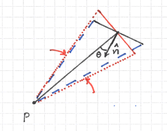
As a result of foreshortening, the solid angle subtended by the patch at \( P \) will appear smaller. This is illustrated in the figure below.

In this figure, the red dotted lines go from \( P \) to the edges of the patch when it is oriented with its normal unit vector parallel to the line-of-sight and the blue dashed lines go from \( P \) to the edges of the patch when it is oriented at an angle \( \theta \) to the line-of-sight. The angle subtended by the red dotted lines is larger than the one subtended by blue dashed lines, so foreshortening effectively reduces the solid angle subtended by the patch.

In differential form, the solid angle of a patch of differential area \( dS \) foreshortened due to observation at an angle \( \theta \) is

$$ d \Omega = \frac{\cos \theta \, dS}{r^2} = \frac{ \left( \hat{r} \cdot \hat{n} \right) dS }{r^2} $$

where \( \hat{r} \) and \( \hat{n} \) are unit vectors.

The solid angle subtended by the patch is obtained by integrating over either expression:

$$ \Omega = \iint_S \frac{\cos \theta \, dS}{r^2} = \iint_S \frac{ \left( \hat{r} \cdot \hat{n} \right) dS }{r^2} $$

Uniformly Sampling Surfaces in Solid Angle

In one of my projects I am working with a rotationally symmetric optical surface that is defined through a recursion relation, but I need a differentiable representation for ray tracing. I obtain this representation by sampling the surface at different polar angles \( \theta \) and fitting the samples with a polynomial or spline.

In some scenarios it is advantageous to uniformly sample the surface in solid angle, rather than angle itself. To achieve this, I uniformly sample \( \cos \theta \) and obtain the values for \( \theta \) by applying an \( \arccos \) function to the samples. In pure Python this looks like the following:

import math


num_samples = 8

# Sample directions from the optical axis to directions perpendicular to it.
cos_theta = [x / (num_samples - 1) for x in range(num_samples - 1, -1, -1)]
assert len(cos_theta) == num_samples

theta = [math.acos(x) for x in cos_theta]

The above code produces values for \( \theta \) of [0.0, 0.5410995259571458, 0.7751933733103613, 0.9625507478846871, 1.1278852827212578, 1.2810446253588492, 1.4274487578895312, 1.5707963267948966].

The reason this works is the following: start with the definition of solid angle \( d \Omega = \sin \theta \, d \theta \, d \phi\). Because the surface is rotationally symmetric, integrate over the azimuthal angle to obtain \( \iint_{\phi = 0}^{2 \pi} \sin \theta \, d \theta \, d \phi = 2 \pi \int \sin \theta \, d \theta \).

But \( \sin \theta \, d \theta = -d ( \cos \theta) \), so uniform sampling in \( \cos \theta \) space produces equal-sized rectangles in the Riemann sum that approximates this integral.

Etendue

Etendue (sorry French speakers) is another important quantity in radiometry. Though it is a core quantity of the science, it is actually a purely mathematical construction and does not require any concept of power, detector, or light source. It is related to solid angle, but is easy to confuse with the above expressions for solid angle because two different patches are involved in its construction, not one.

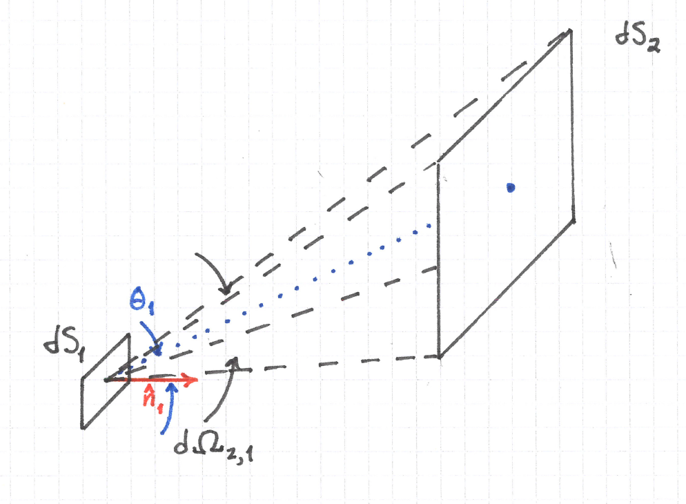
Let \( dS_1 \) and \( dS_2 \) represent these two different surface patches. They are differential patches but drawn unrealistically large in the figure below for ease of understanding. Assume that the solid angle subtended by surface 2 as viewed from the center of surface 1 is \( d \Omega_{2,1} \). Furthermore let \( \theta_1 \) represent the angle between the unit normal vector to \( dS_1 \) and the center of the solid angle \( d \Omega_{2,1} \). Similarly, let \( \theta_2 \) represent the angle between the unit normal vector to \( dS_2 \) and the center of the solid angle \( d \Omega_{1,2} \). Finally, assume these patches sit in a medium with refractive index \( n \).

Etendue is defined as:

$$ dG = n^2 \, \cos \theta_1 \, dS_1 \, d \Omega_{2,1} $$

Conservation of Etendue

We can prove that this quantity is conserved by noting that \( d \Omega_{2,1} = \frac{\cos \theta_2 \, dS_2} {r^2} \), or

$$\begin{eqnarray} dG &=& n^2 \cos \theta_1 \, dS_1 \, d \Omega_{2,1} \\ &=& n^2 \cos \theta_1 \, dS_1 \frac{\cos \theta_2 \, dS_2}{r^2} \\ &=& n^2 \frac{\cos \theta_1 \, dS_1}{r^2} \cos \theta_2 \, dS_2 \\ &=& n^2 \, d \Omega_{1, 2} \cos \theta_2 \, dS_2 \end{eqnarray}$$.

So it does not matter if we measure etendue from surface 1 to surface 2, or from surface 2 to surface 1; it is the same for any two patches.

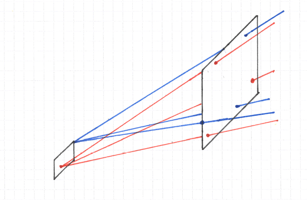
Intuitively, the conservation of etendue is just a fancy way of counting the number of lines that pass through any two patches in space. When viewed this way, it is obvious that the number of lines that pass through both patches must be the same regardless of whether we look from patch 1 to patch 2 or from patch 2 to patch 1.

Phase Space Representation

Rigorously speaking, conservation of etendue is a result of Liouville's theorem. Let each ray be represented in a four dimensional phase space where two dimensions are on a reference surface and the remaining two represent the two degrees of freedom in the optical momentum vector \( \vec{p} = n \hat{s} \) of Hamiltonian optics. The volume of the phase space spanned by all the rays intersecting this surface is a conserved quantity.

Etendue becomes an optical quantity when I assert that the lines represent rays that carry some amount of power \( d \Phi \). Strictly speaking, etendue either stays the same or increases, but it cannot decrease. Diffuse scattering is one way that it can increase, but not because scattering simply redirects light rays. Reflection and refraction also redirect light rays, but in these cases etendue is conserved because reflection and refraction are operations that satisfy Liouville's theorem.

Etendue can be related to the second law of thermodynamics. (But how exactly this is done I do not know.)

A few weeks ago I restarted work on Cherry, my sequential ray tracer, by porting the GUI from Javascript/React to pure WASM with egui. I am very happy with the results. It's much easier to add features with egui, and I have no regrets about giving up the DOM in the web application. I was never very good at web developement, and I always felt that React has too much unseen magic happening behind the scenes.

Having gotten the frontend work out of the way, I turned my attention back to adding features to Cherry. One of the applications that interests me in the lab is scan lenses, i.e. lenses that translate an angular deviation of a laser beam into a lateral displacement. These lenses are designed so that their scanning plane is as flat as possible over a large field of view. They often must work across multiple wavelengths and at large field angles.

As a starting point, I put the f-theta scan lens example from Optiland, which itself comes from Milton Laikin's Lens Design, 4th ed., into Cherry and began varying the incident field angle. It did not take long before problems in the ray tracing routine appeared.

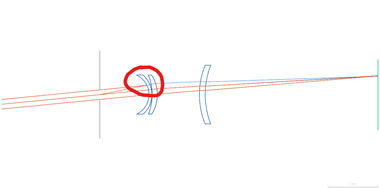
At a field angle of exactly 5.6 degrees, the marginal ray from the Fraunhofer C line ( \( \lambda = 0.6563 \, \mu m\) ) reflects backwards off the first lens surface and intersects the origin. It propagates correctly for field angles of 5.5 degrees and 5.7 degrees, which to me suggests that there is a numerical accident that happens at exactly this value. Furthermore, the spot diagram shows ray-surface intersections across all wavelengths in the image plane disappearing and reappearing randomly as the field angle increases, with the overall number of ray trace errors increasing with field angle. Small angles do not seem to have the problem, and indeed I had not yet tried examples with highly curved surfaces such as this f-theta lens.

As it turns out, the cause of this problem was a silly bug that came from code I wrote three years ago. At the time, I didn't truly and fully understand the Newton-Raphson (NR) root finding algorithm for finding ray-surface intersections. I wanted surface normal vectors to always be unit vectors by convention, and this subtlety ended up degrading and in some cases, ruining the algorithm's ability to find the intersection point, especially at large angles of incidence.

This post is a recap about my journey in debugging the issue and better understanding the NR algorithm. I hope you learn as much as I did from it.

Debugging Ray-Surface Intersections

Running Traces through Algorithms

In practice there are a lot of ray-surface intersections to compute; tracing 1000 rays through 8 surfaces, for example, yields 8000 intersections. This means the algorithm loops 8000 individual times. When only a subset of these fail, it pays to have good debugging tooling in place to identify the state of the algorithm during a failure.

For this I turned to the excellent tracing crate, which has become something of a de facto standard for logging in Rust. The primary abstractions in tracing are events and spans. Events are the most straightforward to understand because they are the same thing as log messages in other languages.

tracing's documentation provides a good, high-level explanation of spans¹:

Unlike a log line that represents a moment in time, a span represents a period of time with a beginning and an end. When a program begins executing in a context or performing a unit of work, it enters that context’s span, and when it stops executing in that context, it exits the span.

The value in using spans is that you can attach data to them, forming a context. Every event that is emitted during a span is associated with this data, regardless of where the event was emitted. In pseudocode, my ray tracing algorithm roughly works like this:

for field in fields.iter():
  for (surface_id, surface) in surfaces.iter().enumerate():
    for (ray_id, ray) in rays.iter().enumerate():
        // coordinate system transformations

        intersect(ray, surface)

        // ray transformations
        // coordinate system transformations

When an intersection failure occurs, I'd like to know the ray_id, but I'd also like to know the state of variables inside the intersection method. Using spans, I do not have to thread ray_id inside the intersect method to attach it to log messages. Instead, I create a span at the top of the inner-most loop that contains ray_id in its context. Then, any events inside the intersection method will be associated to that context. I can then filter by, say, ray_id=42 to see all events that happened for that ray inside intersect().

for field in fields.iter():
  for (surface_id, surface) in surfaces.iter().enumerate():
    for (ray_id, ray) in rays.iter().enumerate():
        let _span = trace_span!("trace_ray", ray_id, surface_id).entered();  // <-- Span begins
        // coordinate system transformations                                        |
                                                                                    |
        intersect(ray, surface)                                                     |
                                                                                    |
        // ray transformations                                                      |
        // coordinate system transformations                                        |
        // <----------------------------------------------------------------------- Span ends

A Failing Test Case

I recreated the same lens in an integration test with a single wavelength at \( \lambda = 0.5876 \) and an off-axis tangential ray fan consisting of 9 rays and incident at 20 degrees. I simplified the test case to reduce the total number of errors, which in turn allowed me to better isolate problems. There were two notable types of errors. In the first, I saw NaNs appear in some of the values manipulated by the Newton-Raphson algorithm:

  2026-03-26T07:49:32.552835Z ERROR cherry_rs::views::ray_trace_3d::rays: Ray intersection did not converge, ctr: 999, s: NaN, residual: NaN
    at cherry-rs/src/views/ray_trace_3d/rays.rs:97

  2026-03-26T07:49:32.552896Z ERROR cherry_rs::views::ray_trace_3d::trace: Ray terminated due to intersection failure, ray_id: 8, surface_id: 2, reason: Ray intersection did not converge
    at cherry-rs/src/views/ray_trace_3d/trace.rs:57

In the second type of error, the ray-surface intersection simply did not converge.

  2026-03-26T07:49:32.553113Z ERROR cherry_rs::views::ray_trace_3d::rays: Ray intersection did not converge, ctr: 999, s: 0.339233626291856, residual: -2.220446049250313e-16
    at cherry-rs/src/views/ray_trace_3d/rays.rs:97

  2026-03-26T07:49:32.553139Z ERROR cherry_rs::views::ray_trace_3d::trace: Ray terminated due to intersection failure, ray_id: 3, surface_id: 3, reason: Ray intersection did not converge
    at cherry-rs/src/views/ray_trace_3d/trace.rs:57

The first type of error was easy to fix. The NaN occurs because the first guess at the intersection point lies further from the axis than the surface's radius of curvature. To correct for this, I now check for NaNs and bisect the guess backwards until I am inside the domain of the surface.

The second error type was the tricky one, and I'll spend the rest of this post discussing it.

The Newton-Raphson Algorithm

At this point while debugging, I began to feel like I needed a refresher in the NR algorithm. It has been about three years since I first implemented it and quite frankly I have forgotten a lot of the details. So I'm going to circle back to the basics to better prepare myself to fix this thing.

Root Finding

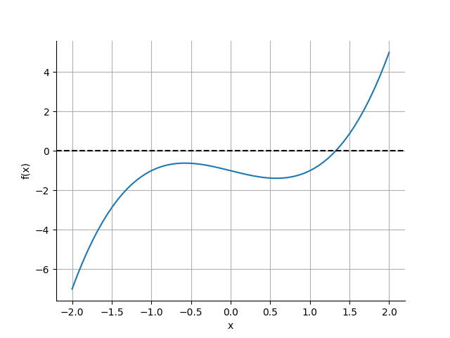
The Newton-Raphson algorithm is a well-known numerical routine for finding the roots (a.k.a. zeros) of a function. I think it's best illustrated by way of example. I found one at https://atozmath.com/example/CONM/Bisection.aspx?q=nr&q1=E1 that involves finding the single zero of the function \( f(x) = x^3 - x - 1 \). The function is plotted below:

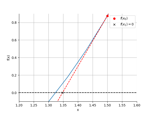
The algorithm is derived as follows: assume we want to find the root of a function \( f(x) \). Choose a starting point \( x_0 \) close to the root and find the slope of the line tangent to the curve of the function at this point. Extend this line to \( x_1 \), the x-intercept where \( y = 0 \). The expression for the slope of \( f (x) \) at \( x_0 \) is

$$ f'(x_0) = \frac{\Delta y}{ \Delta x} = \frac{f(x_0) - f(x_1)}{x_0 - x_1} = \frac{f(x_0) - 0}{x_0 - x_1}. $$

Below you can see what this construction looks like using \( x_0 = 1.5 \).

Solving this expression for \( x_ 1 \) gives

$$ x_1 = x_0 - \frac{f(x_0)}{f'(x_0)}. $$

Repeat the process using \( x_1 \) as the new starting point:

$$ x_2 = x_1 - \frac{f(x_1)}{f'(x_1)}. $$

The more you repeat the process, the closer you get to the root.

Before I Go On, Some Vocabulary

The function \( f(x) \) is often called the residual in the NR literature because it can be thought of as a distance-based error from the the value \( f(x) = 0 \).

As far as I can tell there's no standard term for \( f'(x) \). I'll refer to it as the denominator for simplicity. Once I reach the part of this post on surface representations, I will also refer to it as the surface normal because it is related to the normal vector to the lens surface.

Termination Criteria

There are two common stopping criteria for NR. In the first, you stop iterating whenever the difference between successive steps \( x_i \) and \( x_{i+1} \) is less than some tolerance. In the second, you stop when \( | f(x_n) | \) is less than some tolerance. You can also combine the two so that you stop when either is satisfied. This helps terminate the algorithm when it is converging so slowly that \( \Delta x_i \) is large even but the residual is small.

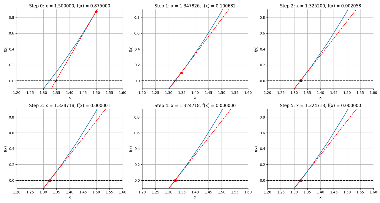
Here are the first six iterations of the algorithm for finding the root of \( f(x) = x^3 - x - 1 \) when starting at \( x_0 = 1.5 \).

After 6 steps, the algorithm has identified the root \( x = 1.324718 \) with a precision better than \( 10^{-6} \).

Oscillations

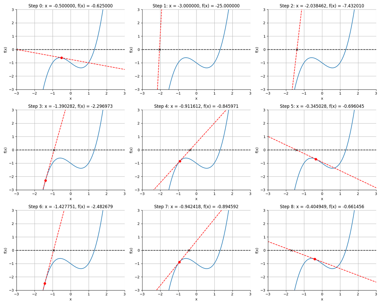
Now of course I deliberately diverted your attention away from the important point that you need to choose the starting point such that it is already close to the root. Here's what happens when I choose a starting point close the local maximum at -0.5:

The algorithm struggles to converge because the initial tangent line is nearly horizontal. This results in the next guess being very far off target and ultimately the algorithm oscillates irregularly around the starting point. However, at step 12, it happens to land just to the right of the local minimum at \( x = 0.7425 \), which sends the next guess far to the right of all local extrema.

From this point, the algorithm can simply descend downhill, where by step 19 it has found the root with a tolerance better than \( 10^{-6} \).

Convergence Guarantees

If the starting point is close to the root, the Newton-Raphson algorithm has quadratic convergence. This means that the error \( \epsilon_{i+1} \) in step \( i + 1 \) is proportional to the square of the error at the previous step, \( \epsilon_i^2 \). But if the starting point is not sufficiently close, then the algorithm can display quite erratic behavior and the assumptions that led to the conclusion about quadratic convergence are no longer valid.

The Importance of the Magnitude of \( f'(x) \)

The preceding discussion demonstrates that the choice of starting point is of great importance. Is there some way to identify a good or bad starting point?

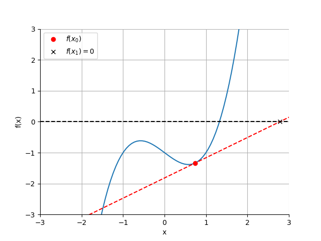
The above figure shows that when the slope of the tangent line is small, the next guess is relatively far away from the current position. Oscillations are more likely to occur when this happens, especially when local extrema are between the trial position and the root.

Conversely, when the slope of the tangent line is large, the next guess is relatively close to the current position. This is what happened with an initial guess of 1.5 as seen here.

We can see this behavior by rewriting the equation for the next guess \( i + 1 \) as:

$$\begin{eqnarray} x_{i+1} &=& x_i - \frac{f(x)}{f'(x)} \\ x_{i+1} - x_i &=& - \frac{f(x)}{f'(x)} \\ \Delta x_i &=& - \frac{f(x)}{f'(x)} \end{eqnarray}$$

So two quantities determine the magnitude of the step. Large step sizes occur when:

1. the residual function \( f(x) \) is large, and
2. the magnitude of \( f'(x) \) is small.

The magnitude of \( f'(x) \) is therefore an indicator of the likelihood of convergence problems. In the extreme case of \( f'(x) = 0 \), the NR algorithm will never converge because of a division by zero in the above equation.

Ray-Surface Intersections

The central problem in ray tracers is to find the 3D intersection of a ray with a surface. The problem has analytical solutions when the surface is planar or spherical, though care must be taken to avoid numerical artifacts such as catastrophic cancellation in their solutions².

When a surface is not flat or spherical, however, we turn to numerical routines such as NR. One early paper describing the approach was from Spencer and Murty in 1962. Spencer and Murty were particularly interested in tracing rays through systems containing general surface shapes like conic section surfaces, aspheres, cylinders, and toroids. They were also interested in an algorithm that would easily accommodate new surface types.

Ray Parameterization

Regardless of whether you use an analytical or numerical solution, you usually approach the problem by first expressing ray propagation in parametric form. I illustrate this construction below:

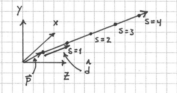
A ray is defined by two, 3D vectors \( \vec{p} \) and \( \hat{d} \). The position vector \( \vec{p} \) points to any point on the ray. \( \hat{d} \) is a vector of unit magnitude whose elements are the direction cosines of the ray. The parameter \( s \) denotes the distance along the ray from the point \( \vec{p} \) so that the set of all points on the ray is expressed as

$$ \vec{r}(s) = \vec{p} + s \hat{d}. $$

When \( s = 0 \), we are at the point \( \vec{p} \) on the ray. Increasing \( s \) moves us in the direction of the ray; decreasing it moves in the opposite direction.

Surface Representations

An implicit representation of a surface in 3D is

$$ F ( x, y, z) = 0. $$

Seen this way, a surface is the zero level set of a 3D scalar function.

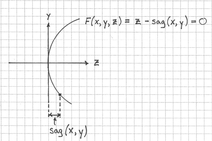
A more useful representation for optical design is to place a single vertex or point of the surface at the origin and let the \( z \) axis represent the optical axis. Let the so-called surface sag, or \( sag(x, y) \), represent the distance from the \( z = 0 \) plane to the surface for all points \( x, y \) within the aperture of the surface³.

We can now rewrite \( F \) as

$$ F(x, y, z) = z - \text{sag}(x, y) = 0 $$.

Saggita for Rotationally Symmetric Conic Section Surfaces

The most common surface types used in optical design are

1. flat surfaces, and
2. rotationally symmetric conic section surfaces, also known as quadrics of rotation.

The surface sag of a flat surface is zero everywhere in the local coordinate system of the surface, which by my definition is the \( z=0 \) plane.

A conic section surface is a surface whose intersection with a plane is a conic section curve, i.e. a circle, parabola, hyperbola, or ellipse. The surface sag of a rotationally symmetric conic section surface with a vertex at the origin and oriented along the \( z \) direction is

$$ \text{sag}(r) = \frac{r^2 C}{1 + \sqrt{1 - (1 + K) C^2 r^2}} $$

where \( r = \sqrt{x^2 + y^2} \) is the radial distance from the origin and \( C \) is the curvature of the surface⁴. It is expressed in terms of curvature and not radius of curvature \( R \) to avoid numeric difficulties with flat surfaces where \( R = \pm \infty \).

The conic constant \( K \) determines the conic's type. The types are defined by:

1. Hyperbola : \( K < -1 \)
2. Parabola : \( K = -1 \)
3. Ellipse : \( K > -1 \)
4. Circle (special case of an ellipse): \( K = 0 \)

The implicit surface representation for a conic section surface is

$$ F (x, y, z) = z - \frac{r^2 C}{1 + \sqrt{1 - (1 + K) C^2 r^2}} = 0 $$.

Partial Derivatives of Rotationally Symmetric Conic Section Surfaces

The last bit of information that I need to calculate ray intersections with conic section surfaces are their partial derivatives. I got these by hand by computing them in polar coordinates and converting them back to Cartesian coordinates using the chain rule. The results are

$$\begin{eqnarray} \frac{\partial F}{ \partial x} &=& \frac{-x C}{\sqrt{1 - (1 + K) C^2 (x^2 + y^2)}} \\ \frac{\partial F}{ \partial y} &=& \frac{-y C}{\sqrt{1 - (1 + K) C^2 (x^2 + y^2)}} \\ \frac{\partial F}{ \partial z} &=& 1 \end{eqnarray}$$

Newton-Raphson for Ray-Surface Intersections

The NR algorithm for computing ray intersections with general surfaces is

$$s_{i+1} = s_i - \frac{F(x,y,z)}{\nabla F (x, y, z) \cdot \hat{d}}.$$

I think most notable is that the denominator has been replaced with the directional derivative of the surface's equation along the direction of the ray's propagation. Another thing worth noting is that \(x\), \(y\), and \(z\) are constrained to lie on the ray by writing \(x = p_x + sl \) and so on for the other two quantities⁵.

At this point I'm at last able to understand where problems in the Newton-Raphson algorithm for ray tracing arise. Remember that oscillations and non-convergence often occur when the derivative of the residual is small or there are local extrema between the starting point and the actual root. In ray tracing, the derivative is expressed as \( \nabla F (x, y, z) \cdot \hat{d} \). This can become small when:

1. A ray is traveling nearly parallel to the surface at a point \( x, y \).
2. The gradient of \( F \) is small.

Geometrical Interpretation of Newton-Raphson Failures

I think the small gradient of \( F \) is more easily understood geometrically. To see this, consider that the \( \nabla F \) is parallel to the surface normal vector at all points on the surface. I can write this as a product of the magnitude of the normal vector and a unit vector pointing in its direction:

$$ \nabla F = |\eta| \hat{\eta}. $$

Now the denominator in the NR update equation is the dot product of the above expression with the direction of the ray, or \( |\eta| \hat{d} \cdot \hat{\eta} \). But both \( \hat{d} \) and \( \hat{\eta} \) are unit vectors, so I can replace their dot product with the cosine of the angle \( \alpha \) between them:

$$ \nabla F \cdot \hat{d} = |\eta| \cos \alpha. $$

So the directional derivative becomes small for large angles of incidence and small normal vectors.

Normal Vectors and Surface Representations

There are two parts of the gradient that can make the denominator in the Newton-Raphson update equation small:

1. The magnitude of the normal vector \( | \eta |\)
2. The angle between the ray direction cosine vector and the unit normal vector \(\hat{d} \cdot \hat{\eta} = \cos \alpha \)

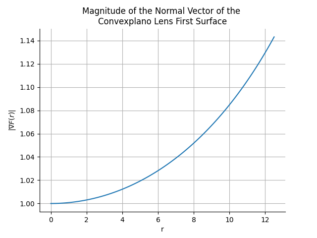
To get a sense of the magnitude of the normal vector, consider the plot of the gradient of \( F \) as a function of radial distance from the vertex of the curved surface of a \(f = 50 \, mm\), 1" diameter, spherical, convexplano lens. The radius of curvature of this surface is 25.8 mm.

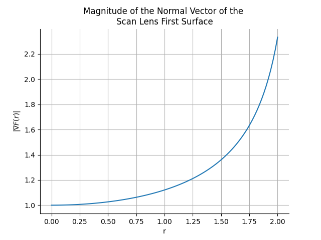
Compare this to the same plot but for the first surface of the scan lens from the beginning of this post, whose radius of curvature is -2.2136 mm.

In neither case is the gradient very small, and we are in some sense rescued by the fact that \( \frac{\partial F}{\partial x} \) is 1 everywhere.

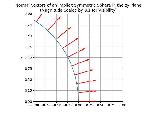
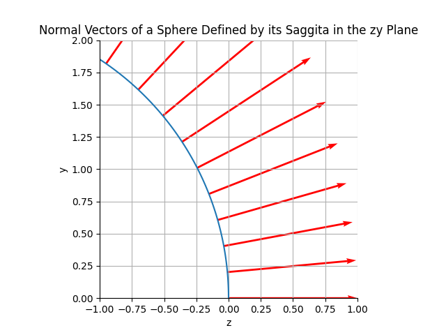
But wait. Shouldn't the normal vector of a spherical surface be a vector of constant magnitude and perpendicular to the surface everywhere? I expected this:

But got this:

So the magnitude of the normal vector varies with distance from the z-axis⁶. And though it's hard to see in these plots, the "normal vectors" are not normal to the surface except at \( x = y = 0 \)!

I was really disturbed by this at first. As it turns out, this is due to representing the surface by its sag, which is effectively a height field above the xy plane. If instead I had used the sphere's symmetric implicit form \(F_s = x^2 + y^2 + (z - R)^2 - R^2 = 0 \) then I would have obtained a normal vector whose magnitude was constant everywhere on the sphere. This is because

$$\begin{eqnarray} \frac{\partial F_s}{ \partial x} &=& 2x \\ \frac{\partial F_s}{ \partial y} &=& 2y \\ \frac{\partial F_s}{ \partial z} &=& 2(z - R). \end{eqnarray}$$

In other words, representing the sphere as a height field has the effect of breaking spherical symmetry with respect to its normal vector⁷.

All of this aside, the magnitude of the normal vector doesn't really become that large in the scan lens example, so the cause of the Newton-Raphson failure is likely coming from near-grazing incidence rays where \(\cos \alpha \approx 0 \).

Back to Debugging

At this point I wanted to confirm that the problematic rays were at near-grazing incidences, so I turned back to the code. Here is a trace of the first five NR iterations of one particular ray that fails to converge at the first surface of the lens:

 2026-04-09T07:25:02.768031Z TRACE cherry_rs::views::ray_trace_3d::rays: intersect_init, pos_x: 3.0616169978683836e-17, pos_y: 0.5, pos_z: -5.0, dir_l: 2.094269368838496e-17, dir_m: 0.3420201433256687, dir_n: 0.9396926207859084, s_init: 5.320888862379561
    at cherry-rs/src/views/ray_trace_3d/rays.rs:69
    in cherry_rs::views::ray_trace_3d::rays::intersect
    in cherry_rs::views::ray_trace_3d::trace::trace_ray with ray_id: 8, surface_id: 2

  2026-04-09T07:25:02.768093Z TRACE cherry_rs::views::ray_trace_3d::rays: newton-raphson iteration data, ctr: 0, s: 4.775443550511577, s_1: 0.0, p_x: 8.633304277606096e-17, p_y: 1.4099255856655057, p_z: -2.5, sag: -0.5071021819862234, residual: -1.9928978180137766, denom: 0.94226
88642314074
    at cherry-rs/src/views/ray_trace_3d/rays.rs:125
    in cherry_rs::views::ray_trace_3d::rays::intersect
    in cherry_rs::views::ray_trace_3d::trace::trace_ray with ray_id: 8, surface_id: 2

  2026-04-09T07:25:02.768118Z TRACE cherry_rs::views::ray_trace_3d::rays: newton-raphson iteration data, ctr: 1, s: 2.8626356840250526, s_1: 4.775443550511577, p_x: 1.306268214832213e-16, p_y: 2.1332978875896096, p_z: -0.5125509346046124, sag: -1.6227826993006131, residual: 1.110
2317646960007, denom: 0.5804199073769454
    at cherry-rs/src/views/ray_trace_3d/rays.rs:125
    in cherry_rs::views::ray_trace_3d::rays::intersect
    in cherry_rs::views::ray_trace_3d::trace::trace_ray with ray_id: 8, surface_id: 2

  2026-04-09T07:25:02.768148Z TRACE cherry_rs::views::ray_trace_3d::rays: newton-raphson iteration data, ctr: 2, s: 4.7418998688939, s_1: 2.8626356840250526, p_x: 9.056747225066086e-17, p_y: 1.479079066939422, p_z: -2.3100023717232365, sag: -0.5666786072973584, residual: -1.74332
3764425878, denom: 0.9276629536509492
    at cherry-rs/src/views/ray_trace_3d/rays.rs:125
    in cherry_rs::views::ray_trace_3d::rays::intersect
    in cherry_rs::views::ray_trace_3d::trace::trace_ray with ray_id: 8, surface_id: 2

  2026-04-09T07:25:02.768181Z TRACE cherry_rs::views::ray_trace_3d::rays: newton-raphson iteration data, ctr: 3, s: 2.997895475725084, s_1: 4.7418998688939, p_x: 1.299243264339216e-16, p_y: 2.1218252727950615, p_z: -0.5440716846947353, sag: -1.5828207424715346, residual: 1.038749
0577767993, denom: 0.5956114914879407
    at cherry-rs/src/views/ray_trace_3d/rays.rs:125
    in cherry_rs::views::ray_trace_3d::rays::intersect
    in cherry_rs::views::ray_trace_3d::trace::trace_ray with ray_id: 8, surface_id: 2

  2026-04-09T07:25:02.768222Z TRACE cherry_rs::views::ray_trace_3d::rays: newton-raphson iteration data, ctr: 4, s: 4.714415826981489, s_1: 2.997895475725084, p_x: 9.340017663658938e-17, p_y: 1.525340640282867, p_z: -2.182899743573678, sag: -0.6094301551576737, residual: -1.57346
95884160044, denom: 0.9166623554823017
    at cherry-rs/src/views/ray_trace_3d/rays.rs:125
    in cherry_rs::views::ray_trace_3d::rays::intersect
    in cherry_rs::views::ray_trace_3d::trace::trace_ray with ray_id: 8, surface_id: 2

In table form:

The denominator is not anywhere near small enough to indicate that the problem is caused by near-grazing incidence angles, so there must be something else going on.

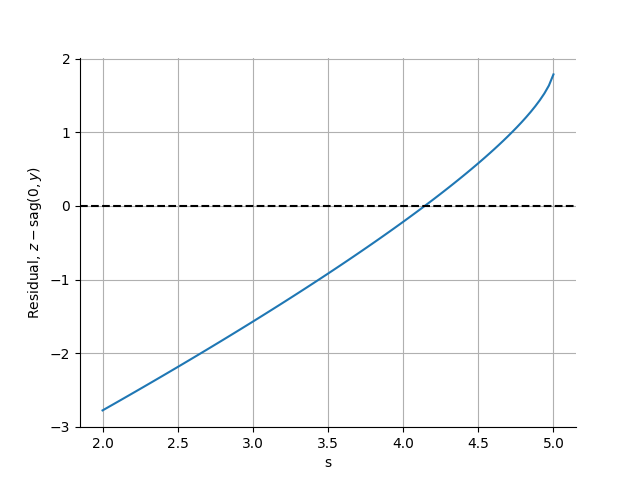
The first thing to note is that the residual \(z - \text{sag} (x, y) \) is oscillating in sign which indicates that the algorithm is hopping back and forth between different sides of the surface. The root estimate s appears to slowly be converging to some value but hasn't yet done so. In fact, it took 100,000 iterations to converge to within 0.0004 of the root, which was somewhere around s=4.14. This rate of convergence is much too slow. What could be causing it?

I plotted the residual function and it didn't seem too bad:

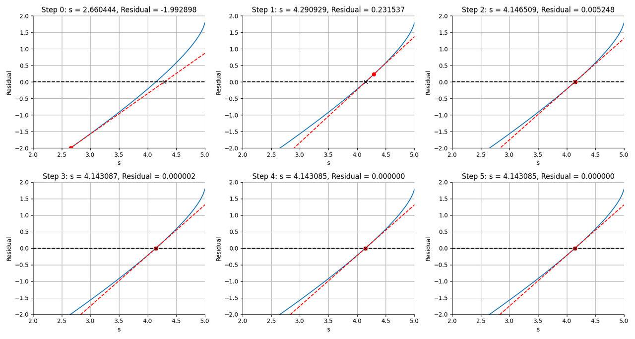
I then plotted the NR steps for this particular ray and found that I could not reproduce the oscillations. In fact, NR converged quite rapidly.

So my two different implementations did not agree. After about 2 hours of digging I found the problem: I was normalizing the normal vector to 1 in the Rust code rather than retaining its magnitude.

// 💣💣💣
let norm = Vec3::new(dfdx, dfdy, dfdz).normalize();
// 💣💣💣

This has a subtle effect on the value of the NR denominator such that the step size isn't quite what it should be.

I can't begin to explain to you how subtle this bug was. I nearly face-palmed by head off when I found it. It was in code that I wrote nearly three years ago. Smart people can do really dumb things with computers.

Discussion

I am actually quite happy to have had to solve this bug even if there was no deeper, numerical reason behind it. It forced me to do a deep dive into the Newton-Raphson algorithm and I feel much more knowledgable as a result. Still, it's frustrating because I clearly was experimenting in the early days, and I wonder whether some other careless coding choices still await to be discovered.

I only briefly mentioned it, but in this journey I also implemented a fallback to a bisection method when the initial NR guess fails due to a negative discriminant in the sag function of a conic section surface. I think this is a win because rays that would have initially failed can be recovered by the fallback routine. But what's more, both of these changes led to some impressive improvements in the benchmark tests: the convexplano lens example runs 43% faster because of faster NR convergence and fewer early ray terminations.

Out of curiosity I looked into what Optiland does to compute Ray-Surface intersections. I believe that it analytically computes intersections for flat and spherical surfaces and falls back to NR when things get more complicated. I use NR for everything, and to be honest, I'm happy with this approach so far. The ray-surface interection function in my ray tracer is a single long function, but it reads linearly and is very clear about what it does. If I were to add if/else branches to check for surface types (or, more properly, employ polymorphism to make the intersection logic a Surface-level method), then the logic would diffuse throughout the codebase. An essay by John Carmack on inlining code that I read a couple years ago had a profound effect on me when it comes to mission-critical, high performance sections of code. Ray-surface intersection logic is one such example where "good" software engineering practices are counter-productive, and just inlining the whole damn thing makes a lot of sense.

The real lesson here is that it always pays to really understand what your algorithms are doing, and having the proper tooling in place for debugging pays off enormously.

Happy ray tracing.

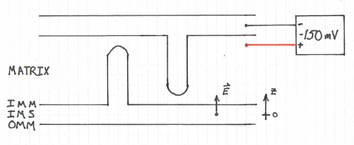
The mitochondrial membrane potential is the potential difference across the inner mitochondrial membrane caused by proton pumps in the electron transport chain. Its value is often cited as about \( -150\, mV \). I can never remember the directional conventions for this, so I made the following sketch as a reminder:

• IMM: Inner mitochondrial membrane
• IMS: Intermembrane space
• OMM: Outer mitchondrial membrane

If you stick the positive lead of a voltmeter inside the mitochontrial matrix and the negative lead in the intermembrane space, you will measure a voltage of about \( -150 \, mV \).

The electric field, which points from positive to negative charge, points from the IMS into the matrix. The definition of potential difference is

$$ \Delta \psi = -\int_C \vec{E} \cdot \, d \vec{\ell} $$

where \( C \) is the path of integration. In the absence of magnetic fields this integral is independent of the path and depends only on the value of the potential at its endpoints:

$$ \Delta \psi = - \left| \vec{E} \right| \times (z_{mat} - z_{ims}) $$

with \( z_{mat} \) and \( z_{ims} \) positions within the matrix and IMS, respectively. This equation also assumes that the electric field is uniform across the membrane, which is clearly a simplification.

The direction of integration is from \( z_{ims} \) to \( z_{mat} \). In the figure above the electric field \( \vec{E} \) and the path length differential \( d \vec{\ell} \) are parallel, so \( \vec{E} \cdot \, d \vec{\ell} \) is positive, and the negative sign in the definition results in a negative value for \( \Delta \psi \).

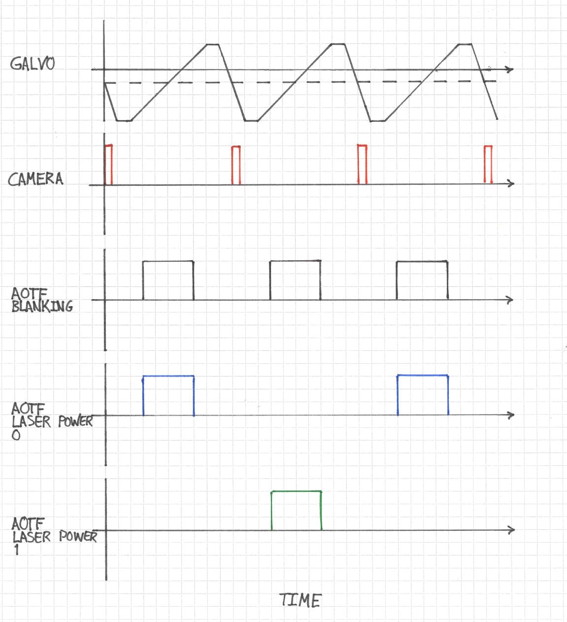
My current project in the lab requires that I update the triggering implementation for an instant structured illumination microscope, or iSIM. The waveforms in the current iteration look like the following:

The most important waveform drives a galvanometric mirror. The timing of this waveform with respect to the camera pulse ensures that the mirror is already in motion and in its linear ramp phase when the camera begins its exposure. Now, the camera is a Photometrics Prime BSI which has a rolling shutter, so "exposure" in this sense refers the period of time during which all rows are exposing, otherwise known as pseudo-global shutter. The acousto-optic tunable filter (AOTF) is configured to interleave two different illumination wavelengths and to expose the sample only during the period of time where the camera is exposing.

For the moment, a National Instruments PCI-6733 DAQ board acts as the leader clock, and all the other components follow it. The board is configured in Python using the nidaqmx package, which is more-or-less a wrapper around the NIDAQmx C API. The goal of this project is to integrate the timing logic into a Micro-Manager (MM) device adapter so that I can remove the Python layer entirely. In doing so, I should be able to harness Micro-Manager's builtin hardware sequencing capabilities so that everything just works after the initial setup.

The main impediment to this goal is a conflict in interfacing the current setup with MM's hardware sequencing model. MM sequencing is based on a state machine, where each trigger signal sequentially advances a hardware device to its next state, eventually looping back to the beginning and starting over. Every device that follows the leader clock needs to be Sequenceable in the MM sense. In the current setup where the NI-6733 is leader, it would have to provide both the clock and entire analog output (AO) waveform for each sequenceable state. This is a much more complex task than simply triggering AO waveforms because interleaving the illumination channels requires different waveforms for different states.

At this point I decided that the problem was too complex to address head on and decided first to address a simpler one: triggering AO waveforms from an external signal.

DAQ Routes

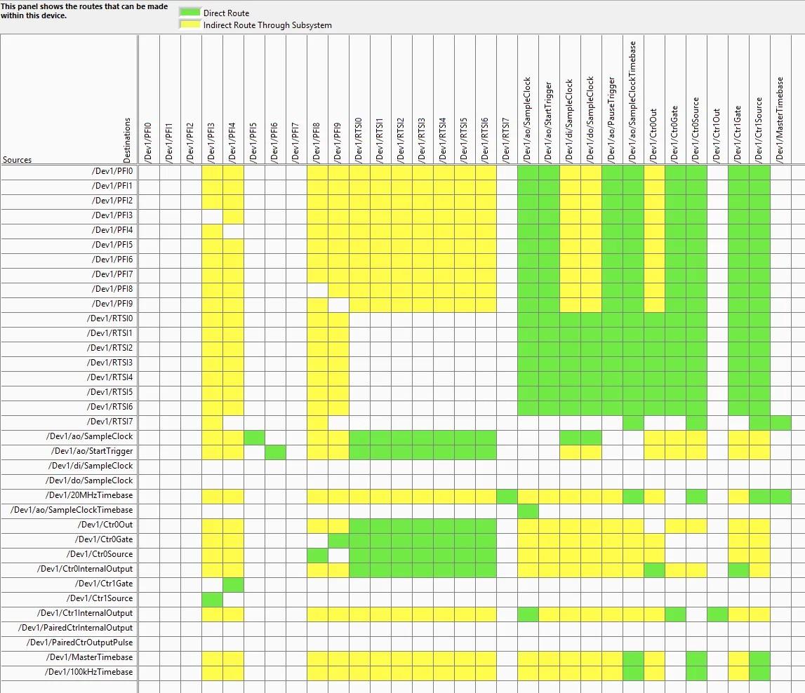
The key to understanding what you can do with your specific NIDAQ board is to access its routing table through the NI MAX software. Here is what the NI-6733 routing table looks like:

Here, Dev1 is the alias for the NI-6733 device. You can see that /Dev1/PFI6 has a direct route to Dev1/ao/StartTrigger. My thinking at this point was that I only need to wire an external trigger source to PFI6 and I should be good to go.

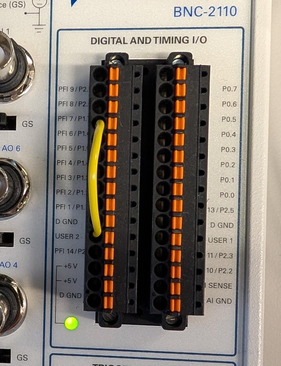
I used the spring terminal and a 22 AWG jumper to connect the USER 2 BNC input to PFI6 on our BNC-2110 interface board as shown here:

For the input trigger I set up a quick push button cirucit using an Arduino Nano to output a 5 V signal on one of the Arduino's digital output pins when the button is pressed. This was fast and good enough for testing.

Finally, I set up a quick NIDAQmx task in Python to wire everything up. I decided to output one period of a 0 - 5 V sinusoid each time the button is pressed.

samples = 1000
t = np.linspace(0, 1, samples) 
waveform = 2.5 + 2.5 * np.sin(2 * np.pi * t)

# Create and configure the task
with nidaqmx.Task() as task:
    # Add analog output channel
    task.ao_channels.add_ao_voltage_chan("Dev1/ao0", min_val=0, max_val=5)

    # #10 kHz sampling rate and 1000 samples => 100 ms sinusoid perid
    task.timing.cfg_samp_clk_timing(
        rate=10000,
        sample_mode=AcquisitionType.FINITE,
        samps_per_chan=samples
    )

    # Configure digital edge start trigger on PFI6, rising edge
    task.triggers.start_trigger.cfg_dig_edge_start_trig(
        trigger_source="/Dev1/PFI6",
        trigger_edge=Edge.RISING
    )

    # Set task to be retriggerable
    task.triggers.start_trigger.retriggerable = True

    # Write waveform to buffer
    task.write(waveform, auto_start=False)

    # Start task (will wait for trigger)
    task.start()

Unfortunately I encountered this error:

nidaqmx.errors.DaqError: Specified property is not supported by the device or is not applicable to the task.

Property: DAQmx_StartTrig_Retriggerable

Retriggerable AO Tasks

As it turns out, the NI-6733 does not support retriggerable AO tasks. This means that, if configured as above, my waveform would only run once. To run it again, I would need to recreate the task in software. This is obviously unacceptable because I need hardware timing.

I found a solution in this NI knowledge base article: https://knowledge.ni.com/KnowledgeArticleDetails?id=kA00Z0000019MXxSAM. The NI-6733's internal counters are retriggerable, and I can use them to serve as the clock for an AO task.

Here's how this works: I setup a NIDAQmx task to output a set number of pulses from one of the counters. The number of pulses is equal to the number of samples in my desired waveform. The counter pulse train is triggered by my 5 V input signal on PFI3.

Next, I rely on a direct connection from the counter's output to the AO channel's clock source . This means that the AO waveform advances by one sample every time a pulse is received from the counter. In terms of the routing table:

• /Dev1/PFI3 --> /Dev1/Ctr1Source
• /Dev1/Ctr1InternalOutput --> /Dev1/ao/SampleClock

The script then creates the two different tasks. NIDAQ devices usually only support running one AO task at a time, but since the counter is not part of AO, I can have both tasks running simultaneously. The full test script is as follows:

import nidaqmx
from nidaqmx.constants import AcquisitionType, Edge, RegenerationMode
import numpy as np
import time

# Generate sinusoid waveform (0 to 5V, 1000 samples)
samples = 1000
t = np.linspace(0, 1, samples)
waveform = 2.5 + 2.5 * np.sin(2 * np.pi * t)

counter_task = nidaqmx.Task()
ao_task = nidaqmx.Task()

try:
    # Configure Counter 1 to generate sample clock pulses
    counter_task.co_channels.add_co_pulse_chan_freq(
        "Dev1/ctr1",
        freq=10000,  # 10 kHz
        duty_cycle=0.5
    )

    # Generate exactly 1000 pulses per trigger
    counter_task.timing.cfg_implicit_timing(
        sample_mode=AcquisitionType.FINITE,
        samps_per_chan=samples
    )

    # Trigger counter from PFI3
    counter_task.triggers.start_trigger.cfg_dig_edge_start_trig(
        trigger_source="/Dev1/PFI3",
        trigger_edge=Edge.RISING
    )

    # Make counter retriggerable
    counter_task.triggers.start_trigger.retriggerable = True

    # Configure analog output task
    ao_task.ao_channels.add_ao_voltage_chan("Dev1/ao0", min_val=0, max_val=5)

    # Use CONTINUOUS mode with external sample clock
    ao_task.timing.cfg_samp_clk_timing(
        rate=10000,
        source="/Dev1/Ctr1InternalOutput",
        sample_mode=AcquisitionType.CONTINUOUS
    )

    # ALLOW regeneration - buffer loops back to beginning
    ao_task.out_stream.regen_mode = RegenerationMode.ALLOW_REGENERATION

    # Write waveform ONCE to buffer
    ao_task.write(waveform, auto_start=False)

    # Start tasks
    ao_task.start()
    counter_task.start()

    print("Tasks configured and running!")
    print("Connect Arduino button to PFI3")
    print("Waveform loaded once - will regenerate on each trigger")
    print("Press Ctrl+C to stop\n")

    try:
        while True:
            time.sleep(0.1)

    except KeyboardInterrupt:
        print("\nStopping tasks...")

finally:
    try:
        ao_task.stop()
        counter_task.stop()
    except:
        pass

    ao_task.close()
    counter_task.close()

Note that regeneration is enabled for the AO task. This means that the waveform is uploaded to the NI-6733's internal buffer and a pointer advances sequentially through it. Once the pointer reaches the end, it circles back to the beginning without having to upload more waveform samples.

Two Color Interleaved Sequential Imaging

I think that this approach can be extended to the original problem of interleaving the different AOTF channels as follows. For the AO task, create a waveform that is two galvo waveform periods long. In the first galvo period, activate the first AOTF channel, and switch to the other channel during the second period.

For the counter, configure a pulse sequence that has half the number of samples as the AO task. So, for example, if the full galvo/camera/AOTF waveform across two periods is 1024 samples, the counter pulse train should be only 512 samples. When it is triggered, it will advance the galvo/etc. waveform by 512 samples and will await the second trigger to advance another 512 samples.

Closing Remarks

The key to setting up complex timing circuits with a NIDAQ is to critically examine its routing table. This can be quite complex, and I found that even my LLM of choice, Claude, made mistakes when interpreting its image. In the end I actually printed it out to examine it on paper.

The other important thing that I learned is that we can use counters to drive other NIDAQmx tasks. This opens up a lot of interesting possibilities, such as the two color interleaved sequencing that I described above.

I am inclined to eventually make the camera the leader in this set up. MM's hardware sequencing works best when this is the case. Additionally, I could free an analog output channel by making this transition.

Finally, I use hard-coded empircal offsets and rely on the agreement between the NIDAQ and camera clocks to ensure that the AOTF signals are applied only during exposure. The Prime BSI camera outputs a signal when all rows are exposing that I am currently not using. It would likely be better to use this expose out signal instead and tie the AOTF timings to this. Doing so would ensure tight synchronization between the AOTF and camera, but the downside would be that it would require a separate hardware controller due to the fact that I can't have more than one AO task running on the NIDAQ at once.

Citation

Yijun Bao and Thomas K. Gaylord, "Clarification and Unification of the Obliquity Factor in Diffraction and Scattering Theories: Discussion," J. Opt. Soc. Am. A 34, 1738-1745 (2017)

Abstract

Two-dimensional (2D) and three-dimensional (3D) diffraction theories form the underlying basis of quantitative phase imaging. This paper reviews how 2D and 3D diffraction theories are developed based on thin and thick object requirements. However, some previously reported work has mixed 2D and 3D theories. This discussion shows that it is possible to enable consistent mixed use of 2D and 3D theories by applying appropriate obliquity factor (OF) modifications. The discussion is concluded with an overall unifying representation for the usage of the OF modifications in 2D and 3D diffraction theories as applied to both thin and thick objects.

Reason for this Review

I often notice that articles concerning quantitative phase imaging (QPI) are unclear about what is meant by 2D and 3D objects. The article helps to clarify this point.

Summary of the Paper

The paper addresses the problem of when to use 2D and 3D diffraction theories in forward models of image formation in a microscope. I will refer to this problem as the choice of dimensionality. In addition, the authors highlight the choice of whether an object may be treated as a "thick" object or a "thin" object, which is not the same as the choice of dimensionality. I call this the choice of object model.

Ultimately, a decision matrix is constructed in which the dimensionality and object model serve as inputs. The output is the form of the obliquity factor, a term found in all diffraction integrals relating to the Huygens-Fresnel principle and that is used to prevent backward energy flow of the wave field¹. The correct forms of the obliquity factor (OF) are then used to allow the application of 2D diffraction theory to thick objects (the so-called Type-1 OF modification) and 3D diffraction theory to thin objects (the Type-2 OF modification).

The unifying theory is meant to address a problem of consistency in the authors' previous work, but I think that it is important on a more fundamental level.

Diffraction Theory

2D Diffraction Theory

2D diffraction theory follows from the well-known developments of Huygens, Fresnel, Kirchoff, Rayleigh, and Sommerfeld. The integral equation for 2D diffraction is:

$$ u ( \vec{x}, z ) = \frac{1}{j \lambda }\int u_{inc} ( \vec{x}', 0) t ( \vec{x}' ) \frac{e^{ j k \sqrt{ (\vec{x} - \vec{x}' ) + z^2 } } }{\sqrt{ (\vec{x} - \vec{x}' ) + z^2 }} K ( \vec{x}, z; \vec{x} ') \, d \vec{x}' . $$

In words, the above expression determines the field \( u \) at transverse coordinate \( \vec{x} \) and axial coordinate \( z \) due to an incident field \( u_{inc} \) on a 2D complex transmission screen \( t \) at \(z = 0 \). \( K \) is the obliquity factor, takes the form \( cos(\theta) \) in the first Rayleigh-Sommerfeld diffraction integral, \( \theta \) being the angle between the normal to the screen and the line from the origin to the point of observation.

This expression is equivalent to Eq. 3-41 of Goodman².

Assumption of the 2D Theory

The most important assumption in 2D diffraction theory is that the object is thin. I think the authors give a somewhat unsatisfactory definition of "thin," stating:

A thin object usually means that the light exits the object approximately at the same transveral coordinate as it enters the object, or the transversal deviation of light can be neglected.

For this definition they cite Goodman². I think they are specifically referring to this passage in Chapter 5, section 1:

With reference to Appendix B, a lens is said to be a thin lens if a ray entering at coordinates (x, y) on one face exits at approximately the same coordinates on the opposite face, i.e. if there is negligible translation of a ray within the lens. Thus a thin lens simply delays an incident wavefront by an amount proportional to the thickness of the lens at each point.

I find the defintion unsatisfactory partly because Goodman is specifically talking about rays and lenses, whereas Bao and Gaylord are talking about waves and inhomogeneous media. At the end of this post I provide a more detailed critique and a possible solution.

Mathematically, this assumption allows us to write the refractive index difference due to the screen as

$$ \Delta n ( \vec{x}, z) = \phi ( \vec{x} ) \delta ( z ) / k $$

where \( \delta \) is the Dirac delta function. The delta function is ultimately the source of the difficulties in reconciling the 2D and 3D theories.

3D Diffraction Theory

By "3D diffraction theory," Bao and Gaylord are referring to what I normally think of as "scattering." In particular, under the first Born approximation:

$$ u ( \vec{r} ) = u_{inc} ( \vec{r} ) + \int u_{inc} ( \vec{r}' ) F ( \vec{ r }' ) G ( \vec{r}, \vec{r}' ) \, d \vec{r}' .$$

This expression states that the total field diffracted (i.e. scattered) by a 3D scattering potental \( F \) is the sum of the incident field and an integral over source terms \( u_{inc} ( \vec{r}') F ( \vec{r}' ) \) multiplied by the Greens function \( G \).

Assumptions of the 3D Theory

In deriving the integral expression above, Born and Wolf³ note in chapter 13 that the gradient of the object's refractive index must be small so that the electric field components can be decoupled, thereby reducing the vector theory to a scalar one. Additionally, the first Born approximation requires that the refractive index contrast of the object be small.

The authors rightly point out that these assumptions are in contradiction with what constitutes a thin object. As a result of the delta function in the expression for \( \Delta n \) of a thin object, the refractive index gradient is huge and 3D diffraction theory should not apply. More specifically, the scalar approximation to the vector Helmholtz equation should be invalid, and it is this approximation that leads to the integral equation of potential scattering.

The authors further state that another consequence of a thin object is that the values of the refractive index become large, which violates the assumption of the first Born approximation. Here I am less certain of their argument, and I think the reason again is due to the nature of the delta function. I think that their argument is this: the refractive index values are large because the delta function technically has an infinite value. But I usually think that the delta function by itself is physically meaningless unless integrated over, which is why I am less certain of the strength of this argument.

An Inconsistency Arises

When applied to a thin object, the two different theories lead to nearly identical expressions for the diffracted field. They differ in that the expression from the 2D theory has an obliquity factor whereas that from the 3D theory does not. The authors point out that this near similarity was discussed in Chapter 1, section 8 of Cowley ¹, a book originally from the 1970's. The authors clarify that the inconsistency arises from "dissimilar object requirements." I think another way to say this is that the assumptions of the 3D theory are violated when applied to a thin object. We will later see that the assumptions are not violated. Rather, the discrepancy comes from incorrectly accounting for the phase accumulated by light incident at an angle to the object.

Conversions between 2D and 3D Theories

Application of 2D theory to 3D objects

In an illuminating (pun intended) discussion the authors proceed to demonstrate that 3D diffraction theory actually emerges from the 2D theory by applying multislice theory. In this theory, a 3D object is divided into many, infinitesimally thin slices and the final field is the sum over the 2D diffracted fields from each slice.

The authors state that, for each slice, both the thin object requirement and the small refractive index contrast requirements are satisfied, which allows for the 2D and 3D theories to be linked. There is an extremely subtle point here because in the previous section the authors stated that an infinitesimally thin slice violates the assumption of small refractive index constrat values. But this is probably because the phase shift of the slice is finite but not infinitesimally small. Here, by making the slices of the 3D object extremely thin, we are also inducing an infinitesimal phase shift in each slice. An infinitesimal phase shift is consistent with the small refractive index contrasts required by the first Born approximation.

Thus the 3D theory can be in a sense rescued by proper and repeated application of the 2D theory.

Now, a proper accounting of the phase shift of each slice must include a division by the obliquity factor:

$$ d \phi ( \vec{x}', z' ) = \frac{ k \Delta n (\vec{x}', z' ) dz' } {K (\vec{x}, z; \vec{x}', z' )} .$$

The logic behind this assertion is that illumination of the slice at an angle results in a larger distance covered in traversing the slice relative to normal illumination. In the words of the authors:

The division of the OF enlarges the effective phase, because the light path length in the slice is \( dz' / K \) for off-axis light.

Combining this with the 2D integral theory results in a cancellation of the obliquity factors and a recovery of the 3D integral expression for the diffracted field.

The authors call this modification to the differential phase imparted by each slice a type I OF modification.

Application of 3D theory to 2D objects

3D theory cannot be applied to 2D objects in an attempt to recover 2D diffraction theory because of the "dissimilar object requirements." By "cannot" the authors really mean "can" because in just a few sentences they circumvent the perceived difficulty by modifying the Greens function in the 3D theory by multiplying by the obliquity factor. This leads to what the authors call a type II OF modification which appears never to have been published before in the literature.

Discussion on the Two Types OF Modification

Section 3C is probably the most important section of the paper. In it, the authors discuss the nature of the proposed OF modifications and why they are justified. By the term "nature," I mean whether they are physically motivated or just mathematical conveniences.

The application of 2D theory to 3D objects is discussed first. The corresponding OF modification to the phase of each slice is physically motivated by "the longer propagation distances of the off-axis rays." The statement at the beginning of the paragraph "A thick object must satisfy [ \( | n ( \vec{r} ) -1 | \ll 1 \) ], which is the requirement of 3D diffraction theory," is a bit puzzling not because of what it asserts (it's correct), but because it seems to imply that a proper application of 2D theory can recover this requirement without having to assume it. But by asserting that we can arrive at the total diffracted field by summing contributions from each infinitesimal slice, we are assuming exactly the first Born approximation. So it is not surprising that we should recover the 3D diffraction theory from multislice modeling when the slices are independent of one another because we made the first Born approximation in assuming the independence of each slice.

Perhaps the authors' intent was just to point out the physical basis of the OF modification to the phase. In this case, I completely agree with the modification and its physical origin.

Next we arrive at a paragraph about why 2D theory cannot be derived from 3D theory. Here the authors state that the phase induced by thin 2D object of thickness \( l \) is \( \phi \approx k l \Delta n \). Since both \( l \) and \( \Delta n \) are small, their product is very small and therefore the object has no appreciable effect on the phase. They next claim that the object cannot satisfy the first Born approximation, which is a bit confusing because the discussion in section 2C seemed to suggest that the problem comes from refractive index values that are too large, not too small.

To be honest, I don't quite follow the logic here, but I again agree with the conclusion. The type II OF modification of the Greens function is just a mathematical convenience that produces the correct results when applying 3D theory to thin objects.

What about the Depth of Field?

Overall, this paper has helped me immensely in understanding the subtleties in the different ways to model diffraction and scattering from transparent objects. In particular, I have a much clearer understanding now on how to properly carry out forward modeling of image formation in high numerical aperture (NA) microscopes.

There is however one significant oversight, which is the definition of what it means for an object to be thin. I find their definition unsatisfactory for the following reason.

Consider a flat piece of glass in air and a ray of light incident upon it. If thin means that "light exits the object approximately at the same tranversal coordinate as it enters the object," then a physically thick piece of glass can be just as "thin" under a small angle of incidence as a physically thin piece of glass under a large angle of incidence. It's the optical path length that matters, not the physical extent of the object.

This is not so much an objection to their definition, but rather to the word "thin" itself. "Thin" alludes to physical extent, but we must remind ourselves that it is really optical extent. But consider next a ray of light that is normally incident upon the glass. Now it doesn't matter how physically thick or thin the glass is; it always exits at the same tranverse coordinate. Is every object under illumination at normal incidence a thin object?

These examples indicate that any defintion of "thin" might have to include the angle of the illumination.

Carrying this example further, if we continuously reduce the NA of the system, then we will measure light that is confined to smaller and smaller angles to the axis. But then we will approach the situation described above where even physically thick objects appear thin under illumination at angles close to normal. Since decreasing the NA increases the depth of field, I suspect that a more satisfactory definition of "thin" will ultimately depend on the depth of field as well.

My hypothesis is that an object's "thinness" really depends on two things:

1. The ratio of its physical extent to the depth of field
2. The refractive index contrast of the object

We need both of the above quantities to be small for an object to be thin.

Conclusion

In conclusion, I really love this paper. It made me critically examine aspects of QPI that I think are taken for granted by clarifying a common point of confusion. Though I might sound critical in this post, it's only because I wish to see the authors' arguments further improved to the point where no ambiguity remains.

The mathematical model of image formation of a thick, transilluminated object by a microscope is complicated yet incredibly interesting. It draws from diverse areas such as crystallography, light scattering, and the theory of partial coherence. I find it much more complicated, but yet more satisfying, than the image formation models of fluorescence microscopy.

This is the first in a series of posts in which I discuss the theory of image formation of a 3D object in brightfield microscopy. The series is inspired by the classic 1985 paper Three-dimensional imaging by a microscope by N. Streibl, but includes a few digressions that I think help to understand subtleties in the theory.

The Problem

The problem is simple: we would like a model that predicts (as much as is possible) the image of a microscopic object that is captured by a brightfield microscope.

Note that this is slightly different from the problem of recovering the object, which cannot be done with complete fidelity in brightfield microscopy.

What is the Object Model?

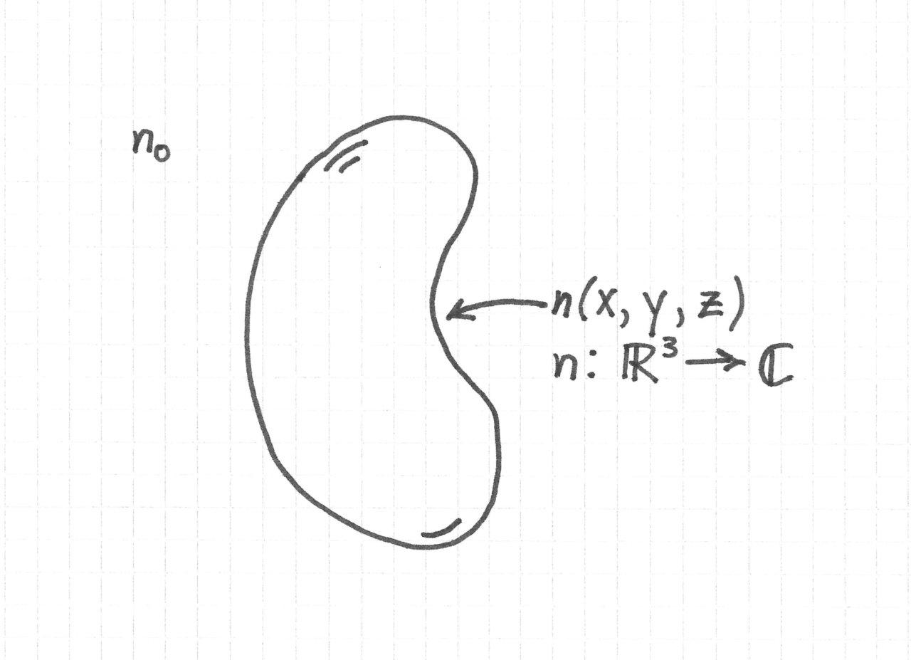
In the theory, the microscopic object, such as a cell or microorganism, is modeled as a complex-valued, three-dimensional function \( n \) of spatial coordinates x, y, and z.

\( n \) is of course the refractive index of the object. The volume outside the object is a uniform medium of refractive index \( n_0 \).

\( n \) is complex to account for

1. phase shifts imparted onto the light, and
2. absorption, which is related to the imaginary part of the refrative index.

Model Classification by Scattering Strength, Object Extent, Depth of Focus

The general model of brightfield image formation is too complex to be of any real use for practical work. As a result, we need to make simplifications to make the theory manageable.

I think that the most useful way to understand these simplifications is by specifying three quantities:

1. The strength of light scattering by the object
2. The object's axial extent
3. The depth of focus of the microscope

We will also need to consider properties such as the coherence of the light source, but I will leave this for a later discussion.

The Scattering Strength and the Object's Axial Extent

The degree of light scattering by an object is the most important characteristic in determining the modeling approach because there is little hope of high-fidelity imaging in strongly scattering samples. (Think of trying to see a distant object in a thick fog¹.)

Roughly speaking, the scattering strength of an object depends on the degree of refractive index variations within the object and the object's extent. All else being equal, a stronger variation of the refractive index within the object leads to stronger scattering. And as the object becomes larger, a larger fraction of the energy carried by the light is scattered light spends more time inside the object.

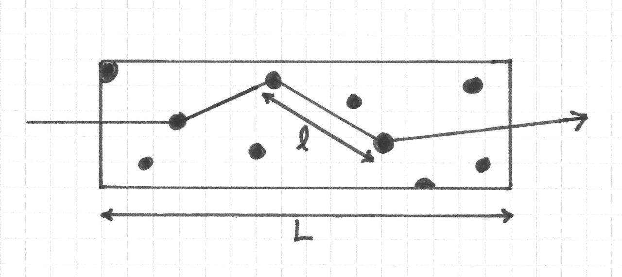
One simple heuristic for the scattering strength is the mean free path of a photon, \( \ell \) inside the object. This is the average distance a photon travels before being scattered. The ratio of \( \ell \) to an object's extent \( L \) is therefore an indication of how many times a photon is likely to scatter.

For weakly scattering objects,

$$ \frac{\ell}{L} \ll 1 $$

I say that this is a heuristic because there are a few problems with this explanation. Namely,

1. As far as I am aware, there isn't a clear relationship between \( \ell \) and the gradient of the refractive index.
2. The mean free path makes sense only if light is modeled as discrete, point-like objects traveling ballistically through the sample, occasionally scattering off of other point-like objects. This is an obvious over-simplification that doesn't reflect the wave nature of light.

Additionally, if the ratio \( \ell / L \) is much less than one, the above picture suggests that light will not interact with the sample at all, but it can still very much diffract.

We'll be dealing with waves and not photons from this point onward, so if you're already experiencing some cognitive dissonance this is part of the reason. Still, this model does help one think about scattering strength without resorting to deeper and much more complicated mathematics, such as the Born approximation and Banach's fixed point theorem.

The Depth of Focus

The depth of focus of the microscope is also important for determining the modeling approach.

Consider the following ratio between the object's axial extent and the microscope's depth of focus, or

$$ \frac{L}{\text{DOF}} $$

The depth of focus is the axial range within which an object appears in focus. When the ratio is significantly less than 1, the object fits entirely within the depth of focus and appears to be effectively two dimensional. When it is about 1 or greater, some sections of the object will appear in focus whereas others will be out-of-focus. The light originating from out-of-focus sections will contribute a nonzero background to the image of the in focus section.

There is no hard cutoff value for this ratio that I am aware of that determines when an object is effectively 2D. Most likely it is more like a continuum where models that assume 2D objects become continuously less accurate as the value of the ratio increases.

In terms of microscope optics, the depth of focus (also confusingly called the depth of field) depends, among other things, on the numerical aperture (NA) of the objective. A higher NA leads to a smaller depth of focus.

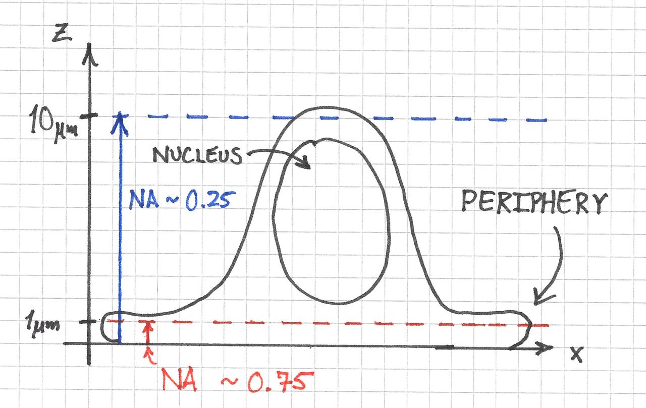
An interesting situation arises when the thickness of an object, such as a cell, varies considerably across its cross section. As illustrated below, a cell might be approximately 2D everywhere when imaged with a 0.25 NA objective, which has an approximately \( 10 \, \mu m \) depth of focus. On the otherhand, only the contents within its periphery would be 2D with a 0.75 NA objective possessing a \( 1 \, \mu m \) depth of focus. Significant portions of the nucleus would be out-of-focus.

Object Modeling Approaches

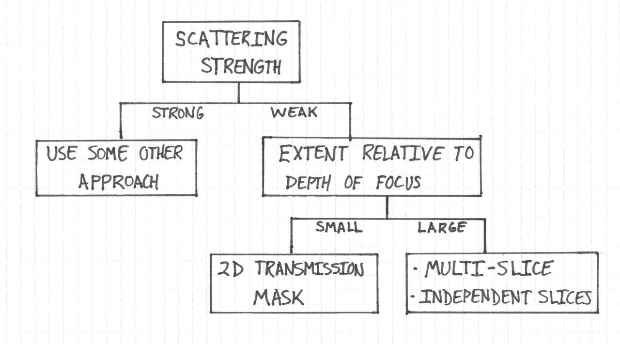
So what are the modeling approaches for the object? I came up with the following decision tree to help explain the process of choosing one, which is further described below.

Strongly Scattering Objects

This is the easiest case. We're probably not going to be doing microscopy for such samples, so we don't even try to model it.

There are techniques other than brightfield microscopy for studying multiply scattering samples, but they are outside the scope of this discussion.

Weakly Scattering Objects

Here we need to know whether the object is larger or smaller than the microscope depth of focus.

Objects Smaller than the Depth of Focus

If the object is smaller than the depth of focus, we can model the sample as a complex 2D transmission mask:

$$ t( x, y) \approx e^{ j k_0 \int \left[ n( x, y, z) - n_0 \right] \, dz } $$

where \( k_0 \) is the free space wavenumber and \( n_0 \) is the refractive index of medium surrounding the object.

This approach effectively projects the small refractive index differences onto a plane transverse to the z-axis. It can be derived from the Helmholtz equation by ignorning transverse gradients of the field's amplitude and approximating the refractive index term, which is quadratic, as a linear function in \( n \).

Objects Larger than the Depth of Focus

One approach to this case is to divide the sample into thin, independent slices. Each slice is modeled as previously described. The final image is obtained by propagating the field from each slice with various degrees of defocus to the image plane, summing the propagated fields, and computing the intensity.

Of course, the slices are really only independent if the scattering is extremely weak. If this is not the case, we could use multi-slice modeling. In this approach, the sample is again divided into thin sequential slices. The difference is that the light diffracted from the first plane serves as the input to the second plane, which diffracts and serves as the input to the third plane, and so on.

Moderately Scattering Samples

I think things get really interesting here, but likely this is best left for later as I don't fully know what options are available.

I will however say that microscopy approaches with optical sectioning, such as confocal and lightsheet, might be of some use.

In the next post I plan on discussing a concept that determines the resolving power of a 3D object under a microscope: the 3D aperture.

The last few months I have been working on developing parametric representations of conic sections so that any arbitrary conic can be drawn to the computer screen. Besides being a fun intellectual exercise, I expect that the performance of the parametric approach should be quite good relative to any iterative method for drawing implicit representations of arbitrary conic curves because no iteration is required.

The parabola in particular has proven to be trickier than I had anticipated, and it has forced me to revisit some of its basic properties.

The Setup

Consider the most general form of a conic curve, which is the implicit equation:

$$ Q ( x, y ) = A x^2 + B x y + C y^2 + D x + E y + F = 0 $$

For a parabola, \( B \) is dependent on the coefficients \( A \) and \( C \) via the equation \( B^2 = 4 A C \), so that the implicit equation for a parabola is

$$ Q ( x, y ) = (a x + c y)^2 + D x + E y + F = 0 $$

where \( a^2 = A \) and \( c^2 = C \).

It can be shown that the axis of symmetry of the parabola is the line

$$ a x + c y + \frac{a D + c E}{2 \left( a^2 + c^2 \right)} = 0 $$

The matrix of the quadratic form for the parabola is

$$\begin{eqnarray} A_{33} = \left( \begin{array}{cc} A & B / 2 \\ B / 2 & C \end{array} \right) = \left( \begin{array}{cc} a^2 & ac \\ ac & c^2 \end{array} \right) \end{eqnarray}$$

\( A_{33} \) is singular and has one eigenvalue whose value is 0.

In this post I show that the eigenvector of the matrix of the quadratic form of a parabola with the zero eigenvalue is parallel to the axis of symmetry.

Determine the Eigenvalues of \( A_{33} \)

The characteristic polynomial of the matrix \( A_{33} \) is

$$\begin{eqnarray} \left( a^2 - \lambda \right) \left( c^2 - \lambda \right) - a^2 c^2 &=& 0 \\ a^2 c^2 - \left( a^2 + c^2 \right) \lambda + \lambda^2 - a^2 c^2 &=& 0 \\ - \left( a^2 + c^2 \right) \lambda + \lambda^2 &=& 0 \end{eqnarray}$$

The solutions to the above equation are \( \lambda = \{ 0, \, a^2 + c^2 \} \).

Find the Eigenvector of the Zero Eigenvalue

The system of equations for finding the eigenvectors is

$$\begin{eqnarray} \left( a^2 - \lambda \right) x + acy &=& 0 \\ acx + \left( c^2 - \lambda \right) y &=& 0 \end{eqnarray}$$

Solving the first equation for \( y \) gives

$$ y = - \left( \frac{a^2 - \lambda}{ac} \right) x $$

Substitute in \( \lambda = 0 \) to find

$$ y = - \left( \frac{a}{c} \right) x $$

The eigenvector is thus

$$\begin{pmatrix} 1 \\ -c / a \end{pmatrix}$$

Recall from above that the axis of symmetry is

$$ a x + c y + \frac{a D + c E}{2 \left( a^2 + c^2 \right)} = 0 $$

This is a line of slope \( m = -a / c \) and is therefore parallel to the eigenvector with the zero eigenvalue.

The Tangent at the Vertex and the Eigenvector with Non-Zero Eigenvalue

The tangent to the parabola at its vertex is perpendicular to the axis of symmetry and must therefore have a slope of \( c / a \)¹.

The eigenvector with eigenvalue \( \lambda = a^2 + c^2 \) of the matrix of the quadratic form is found by substituting this value into the first equation in the system above:

$$\begin{eqnarray} \left( a^2 - \lambda \right) x + ac y &=& 0 \\ -c^2 x + ac y &=& 0 \end{eqnarray}$$

This gives

$$ y = \left( \frac{c}{a} \right) x $$

which is a line whose slope is the negative reciprocal of the slope of the axis of symmetry. The eigenvector with non-zero eigenvalue is therefore parallel to the tangent at the vertex.

For completeness, the eigenvector with non-zero eigevalue is

$$\begin{pmatrix} 1 \\ a / c \end{pmatrix}$$

I am working on rendering cross section views of optical systems for my ray tracer. The problem is one of finding the intersection curve between a plane (the cutting plane) and a quadric surface which represents an interface between two media with different refractive indexes. Quadric surfaces are important primitives for modeling optical interfaces because they represent common surface types in optics, such as spheroids and paraboloids. A pair of quadrics, or a quadric and a plane, models a common lens.

In 3D, the implicit surface equation for a quadric is

$$ A x^2 + B y^2 + C z^2 + D x y + E y z + F x z + G x + H y + I z + J = 0 $$

Any quadric can be reduced to a so-called normal form that identifies its class, i.e. ellipsoid, hyperbolic paraboloid, etc. Except for paraboloids, none of the normal form equations contain linear terms in \( x \), \( y \), or \( z \).

A quadric of revolution occurs when two or more of the parameters of the the quadric's normal form are equal, such as \( x^2 / R^2 + y^2 / R^2 + z^2 / R^2 = 1 \), which is the equation for a spheroid with radius parameter \( R \)¹. Quadrics of revolution are the surface types most-often encountered in optics².

The surface sag of a quadric surface is a very important quantity for ray tracing. The sag of a quadric is usually given in terms of the conic constant, \( K \). One obtains the sag by solving the following quadric equation for \( z \):

$$ x^2 + y^2 - 2 R z + ( K + 1 ) z^2 = 0 $$

Here, \( R \) is the radius of curvature of the surface at its apex, \( x = y = z = 0 \).

At this point I asked myself how I could rewrite the above expression in its normal form, and for a while I was unable to do it. After a bit of searching on the internet, I eventually realized that the solution involves completing the square, a topic that was not given much attention during my high school education. After this exercise, I realize now that the purpose of completing the square is to essentially move any linear terms of a quadratic equation into squared parantheses. This allows one to then remove the linear terms entirely by applying a suitable transformation, leaving only quadratic and constant terms.

Converting the Quadric to its Normal Form

The conversion of the above equation proceeds as follows. We first factor out \( ( K + 1 ) \) from the terms involving \( z \).

$$ x^2 + y^2 + ( K + 1 ) \left[ z^2 - \frac{ 2 R z }{ K + 1 }\right] = 0 $$

Next, we "add zero" to the term inside the square brackets by adding \( [ 2 R / 2 ( K + 1 ) ]^2 - [ 2 R / 2 ( K + 1 ) ]^2 = [ R / ( K + 1 ) ]^2 - [ R / ( K + 1 ) ]^2 \):

$$ x^2 + y^2 + ( K + 1 ) \left[ z^2 - \frac{ 2 R z }{ K + 1 } + \left( \frac{ R }{ K + 1 } \right)^2 - \left( \frac{ R }{ K + 1 } \right)^2 \right] = 0 $$

We can understand this a bit more generally by considering the expression \( z^2 - a z \). Here I need to add and subtract \( ( a / 2 )^2 \). The reason is that now we can rewrite the first three terms inside the square brackets as a squared binomial:

$$ x^2 + y^2 + ( K + 1 ) \left[ \left( z - \frac{ R }{ K + 1 } \right)^2 - \left( \frac{ R } { K + 1 } \right)^2 \right] = 0 $$

These last two steps complete the square. To place the equation into its normal form, I apply the Euclidean transformation \( z' = z - \frac{ R }{ K + 1 } \) and carry through the \( K + 1 \).

$$ x^2 + y^2 + ( K + 1 ) z^{ \prime 2 } - R^2 / ( K + 1 ) = 0 $$

The above equation is almost a normal form expression for a quadric. To finish the job, I would need to substiute in a specific value for the conic constant and divide through so that the constant is either -1, 0, or 1.

As a microscopist I work with very weak light signals, often just tens of photons per camera pixel. The images I record are noisy as a result¹. To a good approximation, the value of a pixel is a sum of two random variables describing two different physical processes:

1. photon shot noise, which is described by a Poisson probability mass function, and
2. camera read noise, which is described by a Gaussian probability density function.

Read noise has units of electrons, which must be discrete, positive integers. So why is it modeled as a continuous probability density function²?

The Source(s) of Read Noise

Janesick³ defines read noise as "any noise source that is not a function of signal." This means that there is not necessarily one single source of read noise. It is commonly understood that it comes from somewhere in the camera electronics, but "somewhere" need not imply that it is isolated to one location.

The signal from a camera pixel is the number of photoelectrons that were generated inside the pixel. I imagine readout of this signal as a linear path consisting of many steps. The signal might change form along this path, such as going from number of electrons to a voltage. At each step, there is a small probability that some small error is added to (or maybe also removed from?) the signal. The final result is a value that differs randomly from the original signal.

Importantly, I do not think that it matters which physical process each step actually represents; rather there just has to be many of them for this abstraction to be valid.

"But aren't there only a handful of steps?" you might ask. After all, linear models of photon transfer typically consist of a few processes such as detection, amplification, readout, and analog-to-digital conversion. I am not referring to these when I use the term "step." Rather, I am referring to processes that are much more microscopic, such as passage of a signal through a transistor or amplifier chip. At the very least Johnson noise, or random currents induced by thermal motion of the charge carriers, will be present in all of the camera's components.

Read Noise is Gaussian because of the Central Limit Theorem

The reason for my conclusion that I can ignore the details so long as there are many steps is the following:

I can model the error introduced by each step as a random variable. Let's assume that each step is independent of the others. The result of camera readout is a sum of a large number of independent random variables. And of course the Central Limit Theorem states that the distribution of the sum of random variables tends towards a normal distribution, i.e. Gaussian, as the number of random variables tends towards infinity. This happens regardless of the distributions of the underlying random variables.

So read noise can appear to be effectively Gaussian so long as there are many steps along the path of conversion from photoelectrons to pixel values and each step has a chance of introducing an error.

Sums of Discrete Random Variables

I encountered one conceptual difficulty here: the sum of discrete random variables is still discrete. If I have several variables that produce only integers, their sum is still an integer. I cannot get, say, 3.14159 as a result. Does the Gaussian approximation, which is for continuous random variables, still apply in this case?

This question is relevant because the signal in a camera is transformed between discrete a continuous representations at least twice: from electrons to voltage and from voltage to analog-to-digital units (ADUs).

Let's say that I have a discrete random variable that can assume values of 0 or 1, and the probability that the value is 1 is denoted \( p \). This is known as a Bernoulli trial. Now let's say that I have a large number \( n \) of Bernoulli trials. But the sum of \( n \) Bernoulli trials has a distribution that is binomial, and this is well-known to be approximated as a Gaussian when certain conditions are met, including large \( n \)⁴. So a sum of a large number of discrete random variables can have a probability distribution function that is approximated as a Gaussian.

This does not mean that the sum of discrete random variables can take on continuous values. Rather, the probability associated with any one output value can be estimated by a Gaussian probability density function.

But how exactly can I use a continuous distribution to approximate a discrete one? After all, if the random variable \( Y \) is a continuous, Gaussian random variable, then \(P (Y = a) = 0 \) for all values of \( a \). To get a non-zero probability from a probability density function, I need to integrate it over some interval of its domain. I can therefore integrate the Gaussian in a small interval around each possible value of the discrete random variable, and then associate this integrated area with the probability of the obtaining that discrete value. This is called a continuity correction.

Example of a Continuity Correction

As a very simple example, consider a discrete random variable \( X \) that is approximated by a Gaussian continuous random variable \( Y \). The probability of getting a discrete value 5 is \( P (X = 5) \). The Gaussian approximation is \( P ( 4.5 \lt Y \lt 5.5 ) \), i.e. I integrate the Gaussian from 4.5 to 5.5 to compute the approximate probability of getting the discrete value 5.